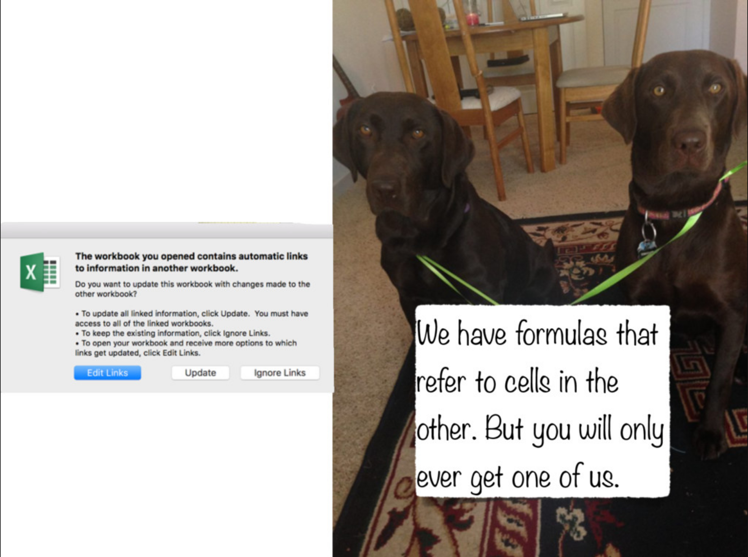
Why Not Excel? I
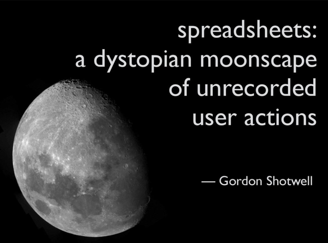
Why Not Excel? II
Why Use R?
Free and open source
A very large community
- Written by statisticians for statistics
- Most packages are written for
Rfirst
Can handle virtually any data format
Makes replication easy
Can integrate into documents (with
R markdown)R is a language so it can do everything
- A good stepping stone to learning other languages like Python

Excel and Stata Can't Do This (In Slides)
library("gapminder")library("tidyverse")ggplot(data = gapminder, aes(x = gdpPercap, y = lifeExp, color = continent))+ geom_point(alpha=0.3)+ geom_smooth(method = "lm")+ scale_x_log10(breaks=c(1000,10000, 100000), label=scales::dollar)+ labs(x = "GDP/Capita", y = "Life Expectancy (Years)")+ facet_wrap(~continent)+ guides(color = F)+ theme_light()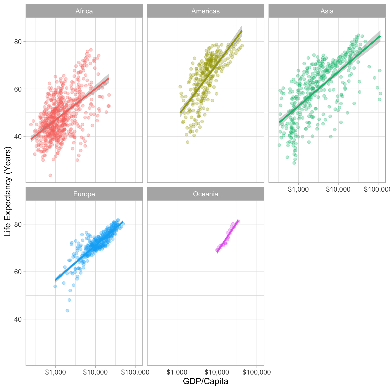
R and R Studio I
R is the programming language that executes commands
R Studio is an integrated development environment (IDE) that makes your coding life a lot easier
- Write code in scripts
- Execute individual commands or entire scripts
- Auto-complete, highlight syntax
- View data, objects, and plots
- Get help and documentation on commands and functions
- Integrate code into documents with
R Markdown
R Studio
R and R Studio II
R is like your car's engine, R Studio is the dashboard
You will do everything in R Studio
R itself is just a command language (you could run it in your computer's shell/terminal/command prompt)
R Studio
R and R Studio III
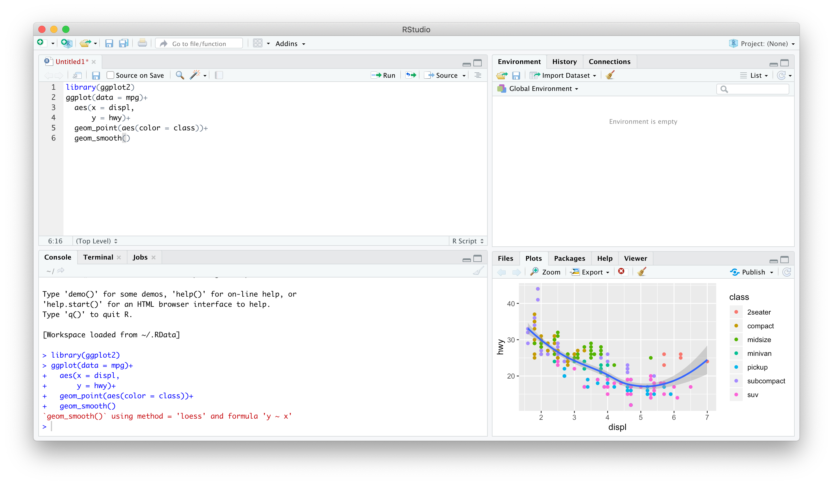
R Studio has 4 window panes:
- Source†: a text editor for documents, R scripts, etc.
- Console: type in commands to run
- Browser: view files, plots, help, etc
- Environment: view created objects, command history, version control
R Studio
†May not be immediately visible until you create new files.
...and Sucking

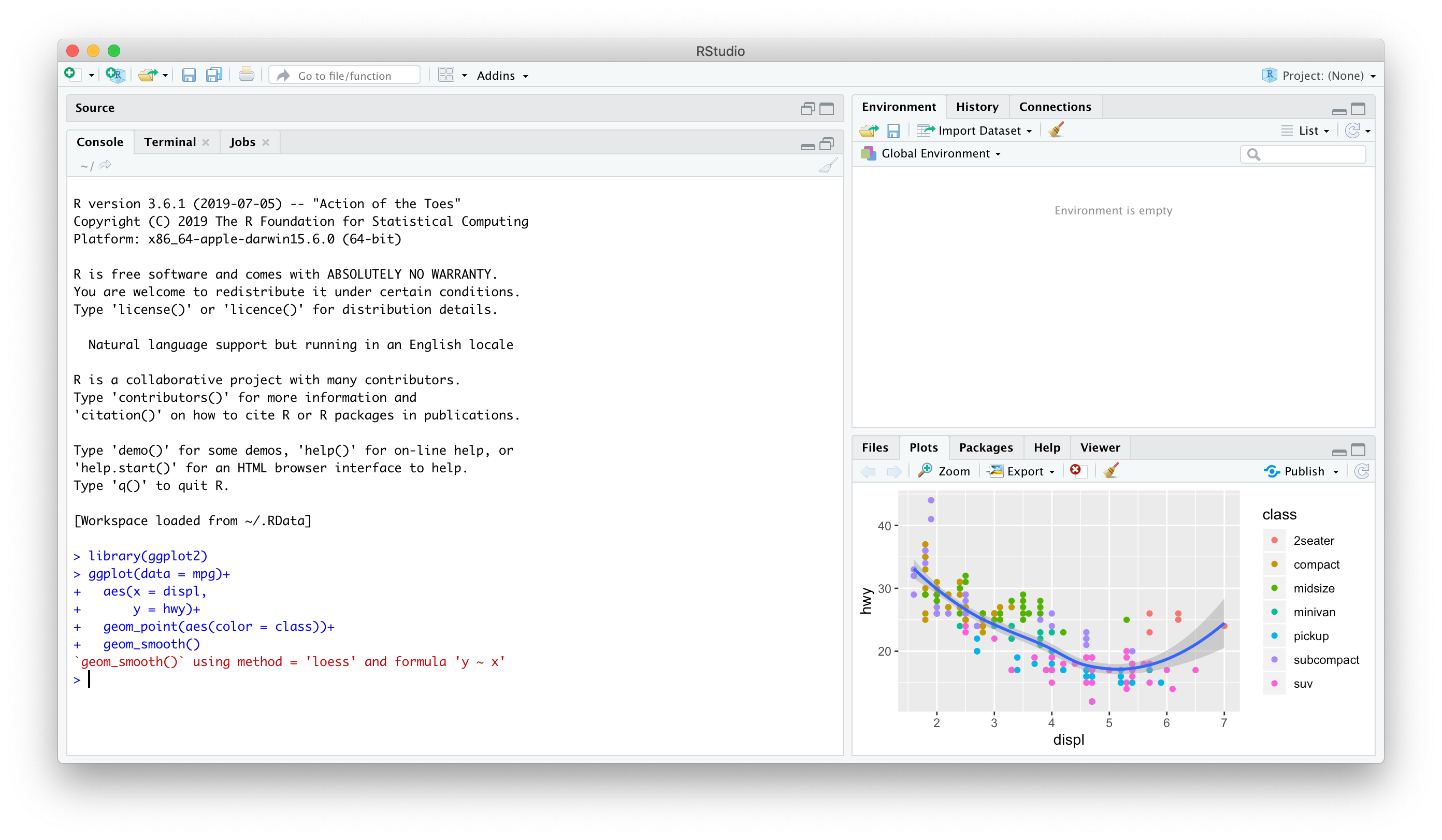
1. Using the Console
Type individual commands into the console window
Great for testing individual commands to see what happens
Not saved! Not reproducible! Not recommended!
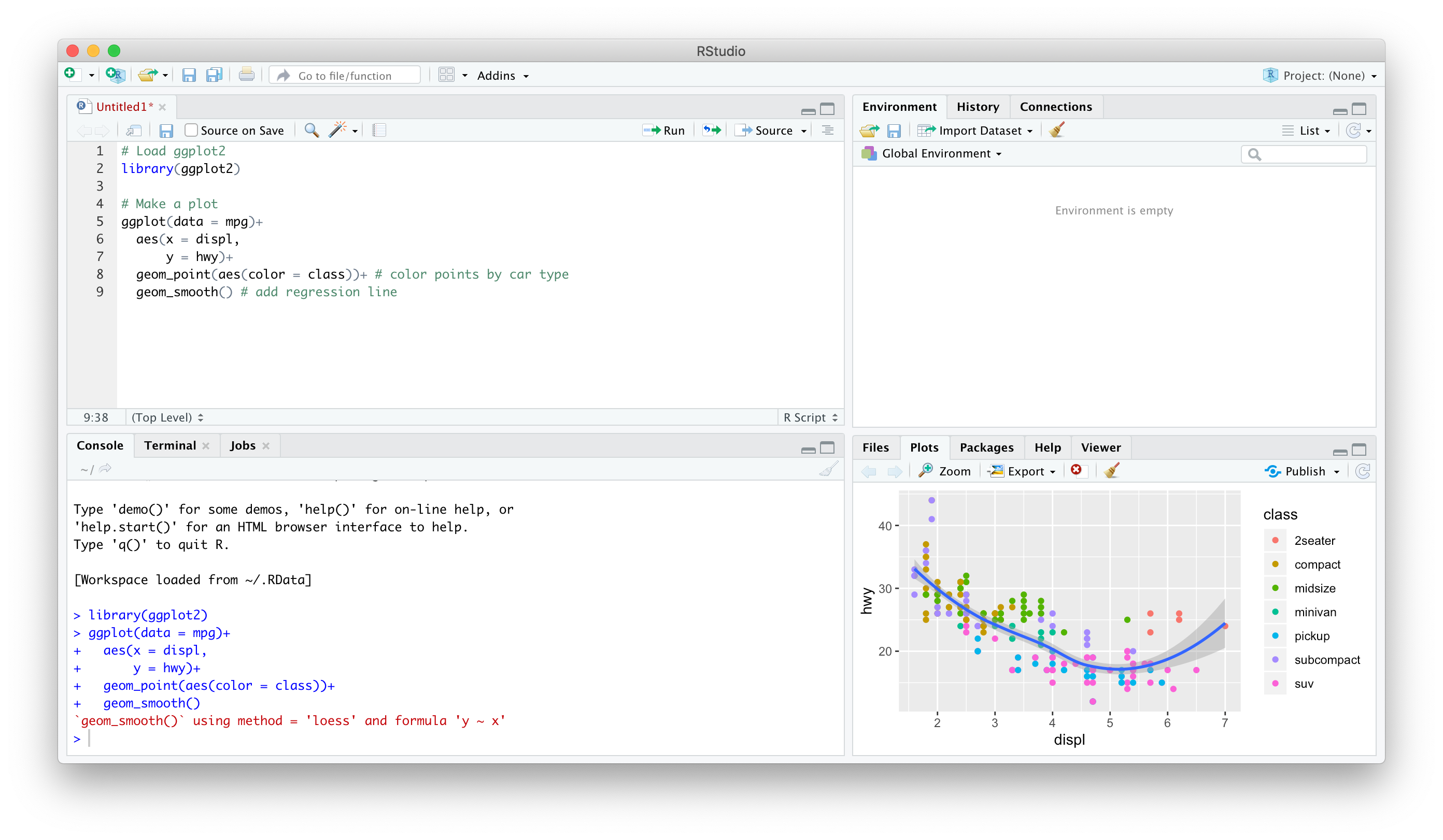
2. Writing an R Script
Source pane is a text-editor
Make
.Rfiles: all input commands in a single scriptComment with
#Can run any or all of script at once
Can save, reproduce, and send to others!
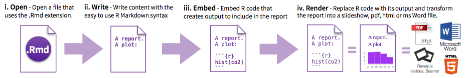
3. Using Markdown
A later lecture:
R Markdown, a simple markup language to write documents in- Optional, but many students have enjoyed it and use it well beyond this class!
Can integrate text,
Rcode, figures, citations & bibliographies in a single plain-text file & output into a variety of formats: PDF, webpage, slides, Word doc, etc.
Coding

Hadley Wickham
Chief Scientist, R Studio
"There’s an implied contract between you and R: it will do the tedious computation for you, but in return, you must be completely precise in your instructions. Typos matter. Case matters." - R for Data Science, Ch. 4
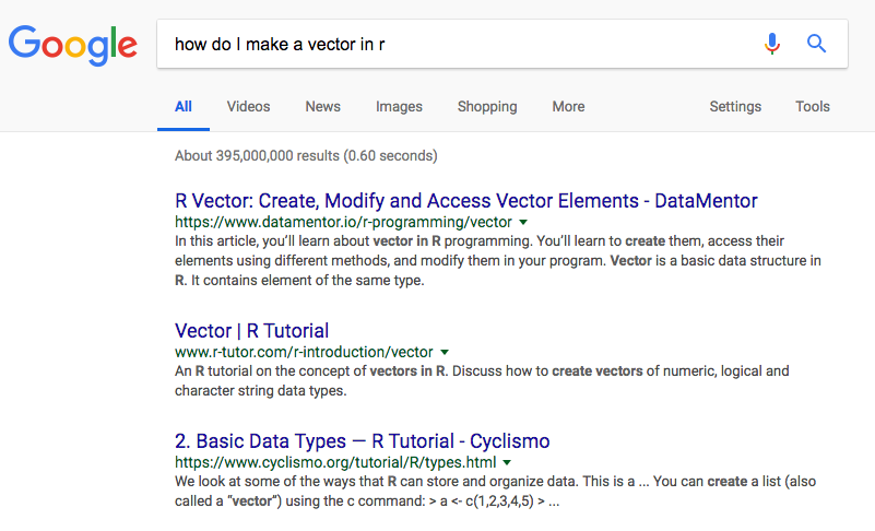
Say Hello to My Little Friend
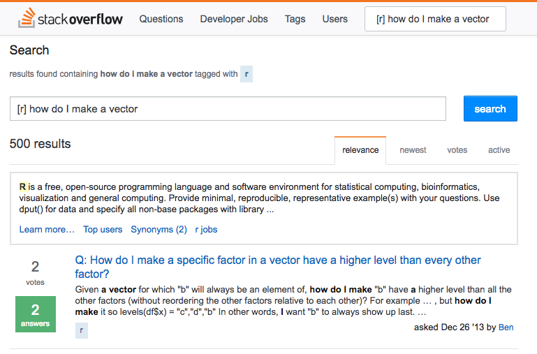
Say Hello to My Better Friend
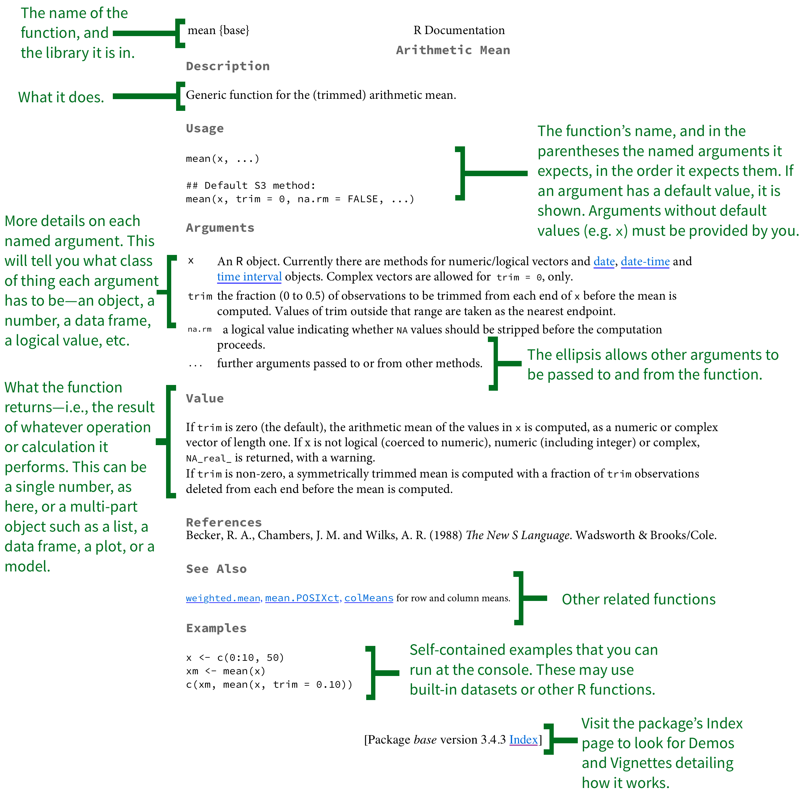
R Is Helpful Too!
- type
help(function_name)or?(function_name)to get documentation on a functionFrom Kieran Healy's excellent (free online!) book on Data Visualization.
]
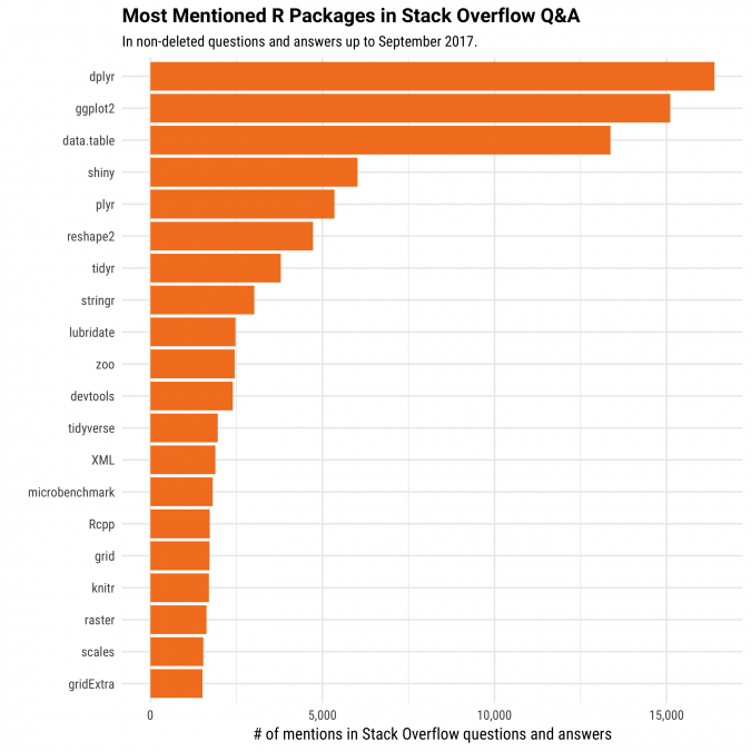
Packages
- Since R is open source, users contribute packages
- Really it's just users writing custom functions and saving them for others to use
- Load packages with
library()- e.g.
library("package_name")
- e.g.
- If you don't have a package, you must first
install.packages()†- e.g.
install.packages("package_name")
- e.g.
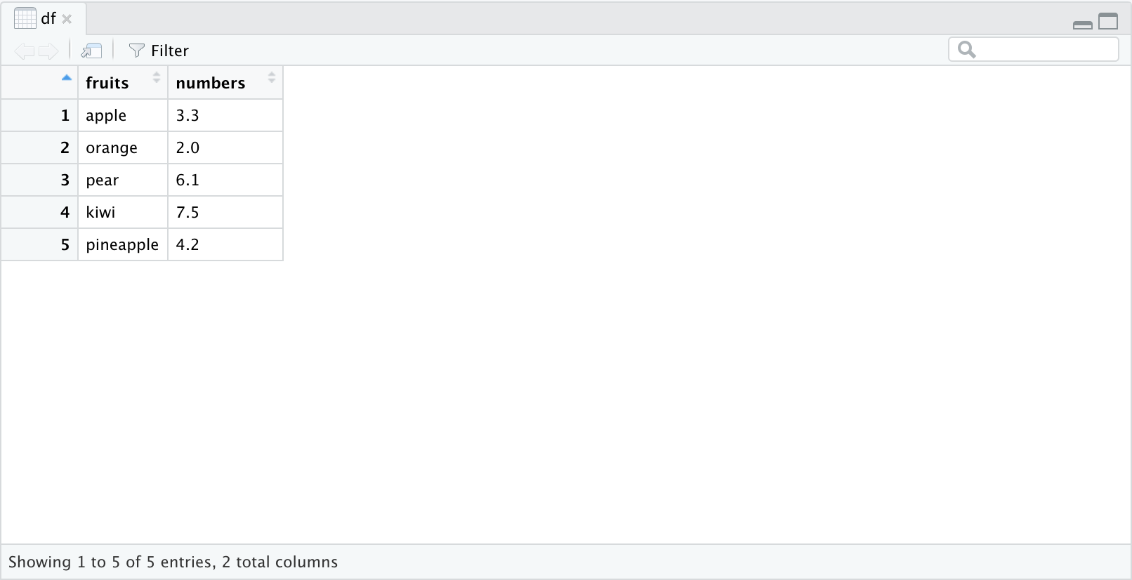
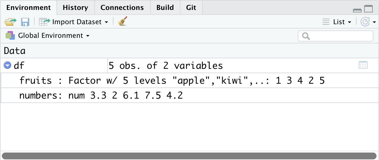
More on Data Frames IV
- Note, once you save an object, it shows up in the Environment Pane in the upper right window
- Click the blue arrow button in front of the object for some more information
More on Data Frames V
data.frameobjects can be viewed in their own panel by clicking on the name of the object in the environment pane- Note you cannot edit anything in this pane, it is for viewing only