Plotting in Base R: Histogram
- Using the
mpgdata, plotting a histogram ofhwy
hist(mpg$hwy)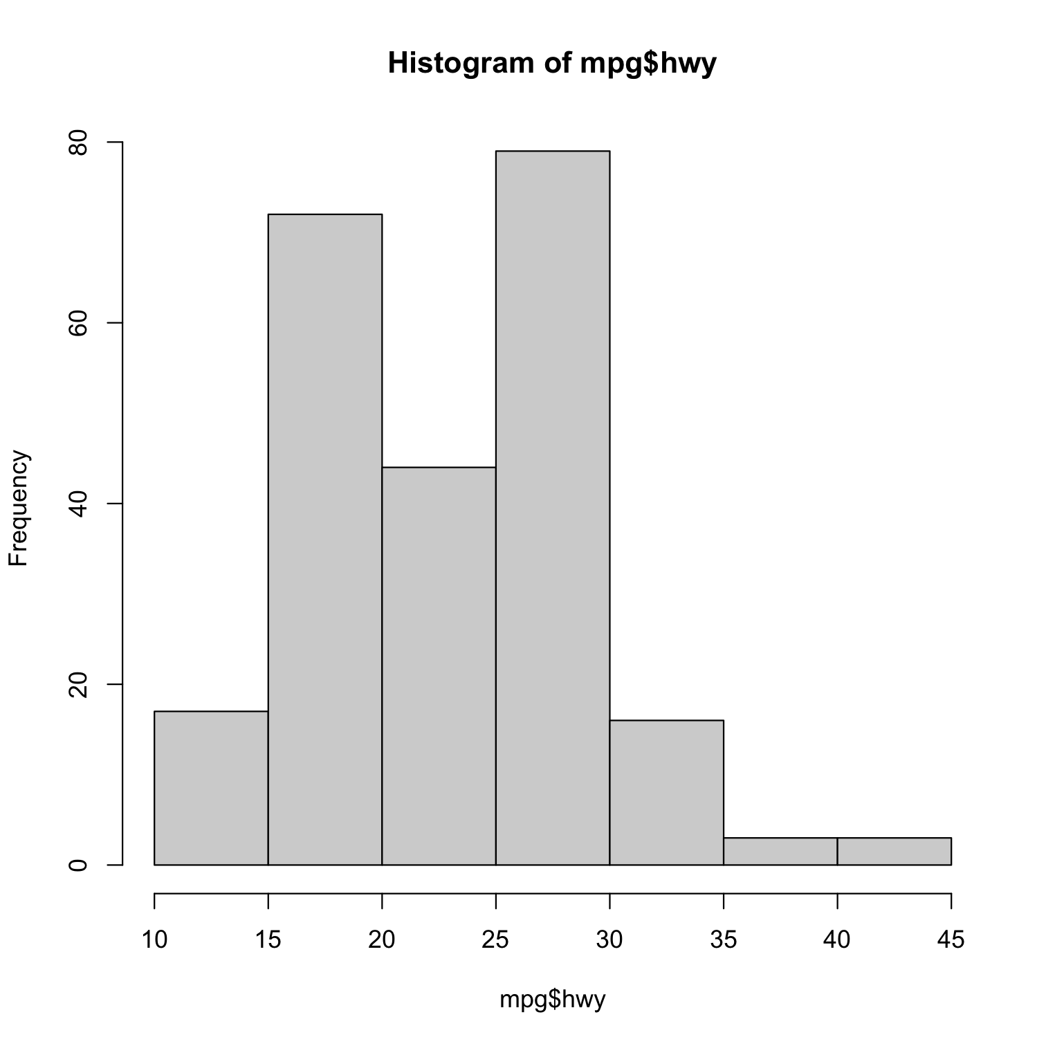
Plotting in Base R: Boxplot
- Using the
mpgdata, plotting a boxplot ofhwy
boxplot(mpg$hwy)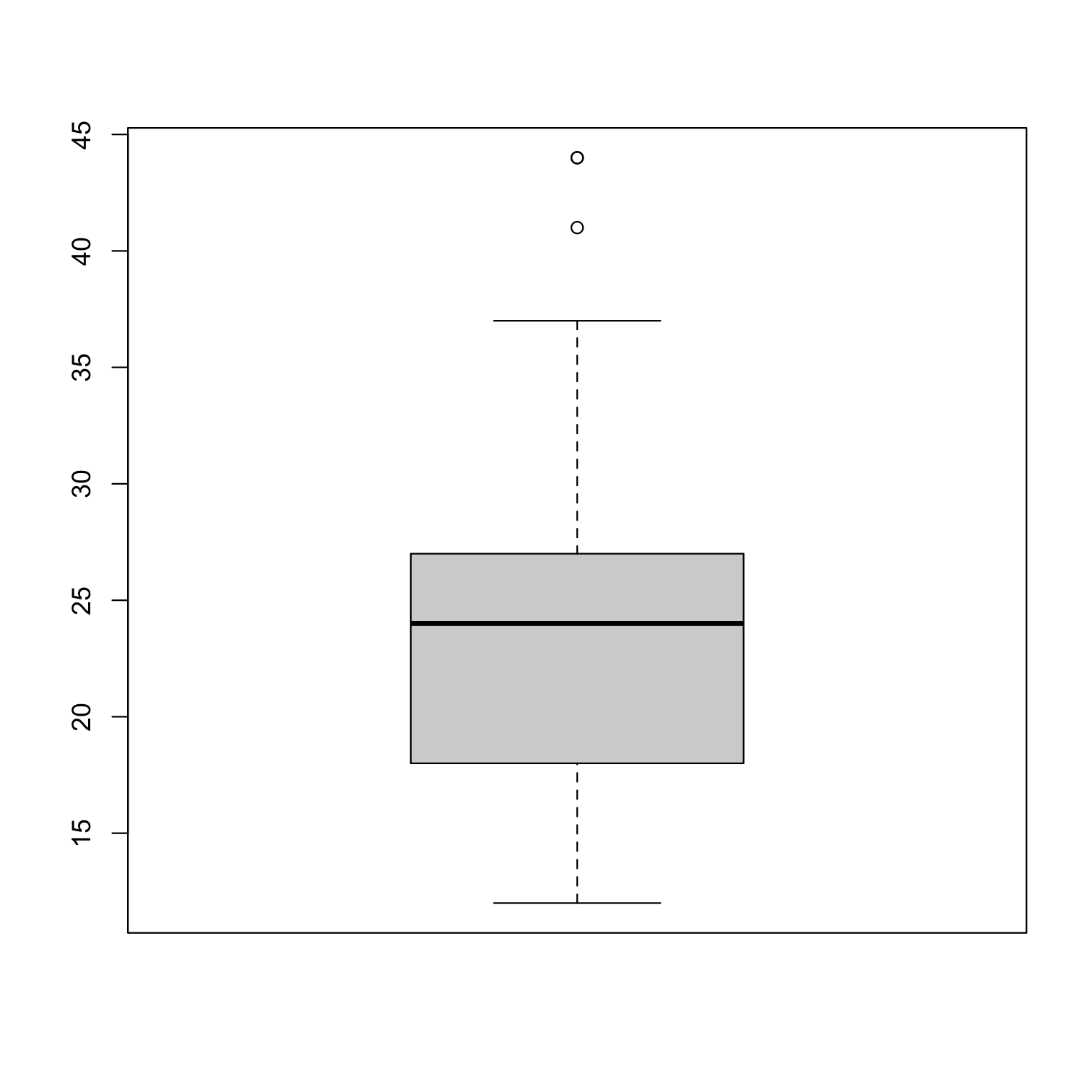
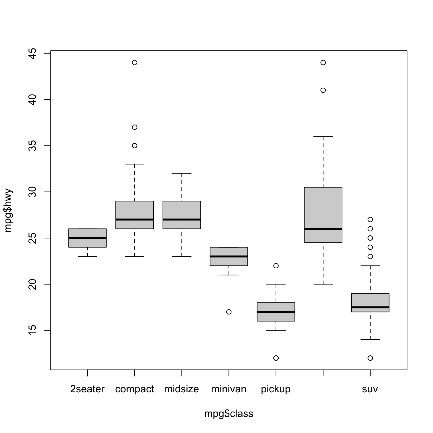
Plotting in Base R: Boxplot by Category
- Using the
mpgdata, plotting a boxplot ofhwybyclass
boxplot(mpg$hwy ~ mpg$class)# second methodboxplot(mpg ~ class, data = mtcars)- The
~is part ofR's “formula notation”:- Dependent variable goes to left
- Independent variable(s) to right, separated with
+'s - Think
y~x+zmeans "yis explained byxandz"
Plotting in Base R: Scatterplot
- Using the
mpgdata, plotting a scatterplot ofhwyagainstdispl
plot(mpg$hwy ~ mpg$displ)# second methodplot(hwy ~ displ, data = mpg)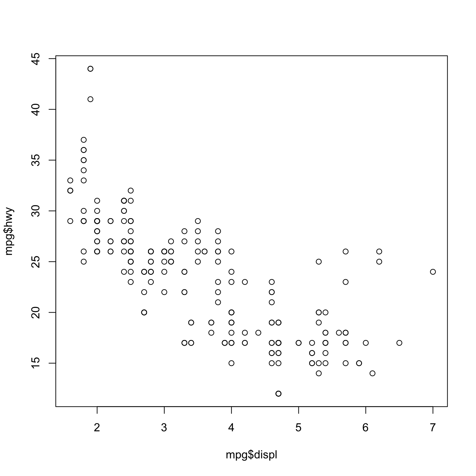
The tidyverse
"The tidyverse is an opinionated collection of R packages designed for data science. All packages share an underlying design philosophy, grammar, and data structures.
Largely (but not only) created by Hadley Wickham
We will look at this much more extensively next week!
This "flavor" of
Rwill make your coding life so much easier!

ggplot
ggplot2is perhaps the most popular package inRand a core element of thetidyverseggstands for a grammar of graphicsVery powerful and beautiful graphics, very customizable and reproducible, but requires a bit of a learning curve
All those "cool graphics" you've seen in the New York Times, fivethirtyeight, the Economist, Vox, etc use the grammar of graphics


ggplot: All Your Figure are Belong to Us
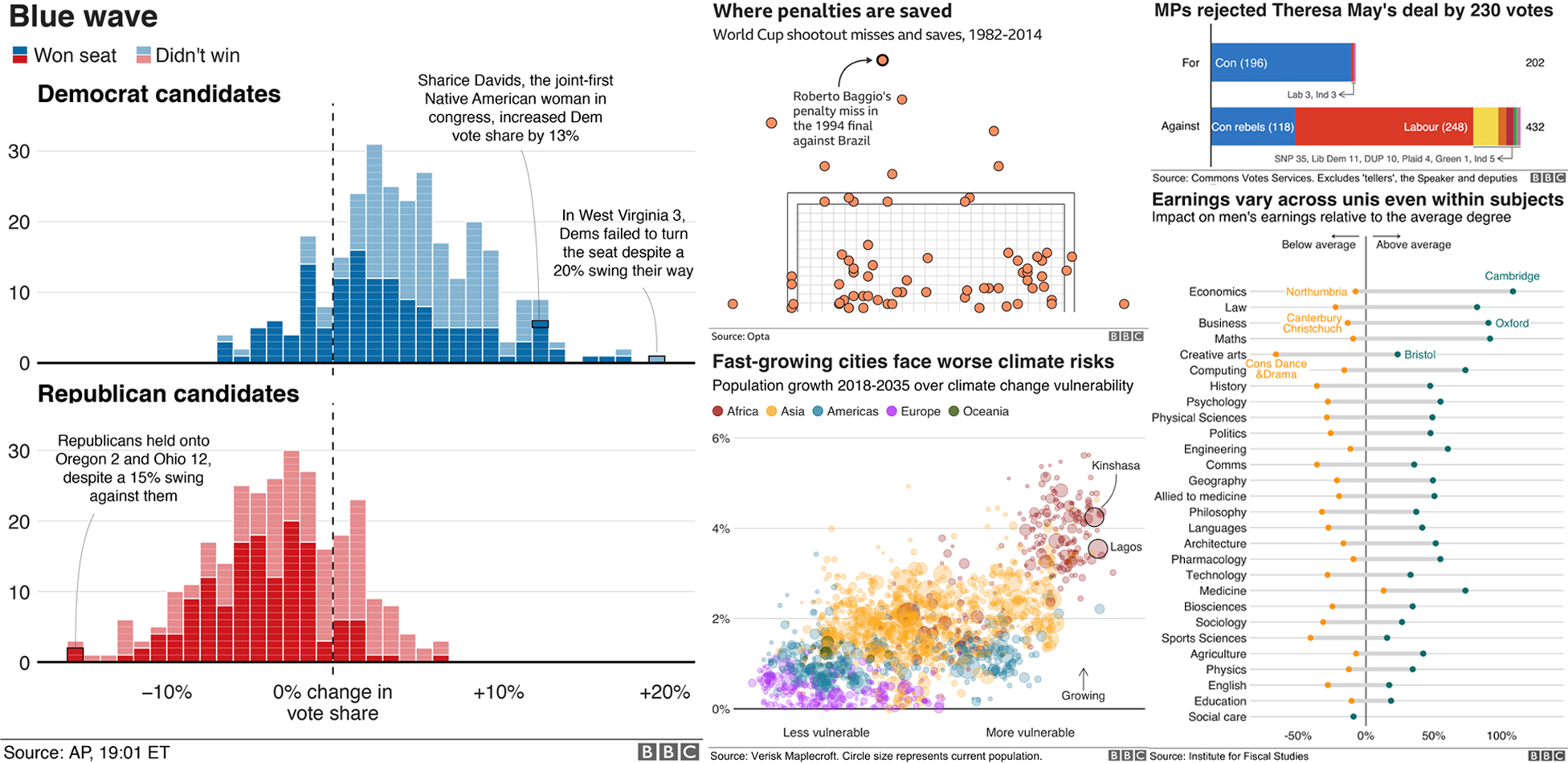
Source: BBC's bbplot
Why Go gg?

Hadley Wickham
Chief Scientist, R Studio
"The transferrable skills from ggplot2 are not the idiosyncracies of plotting syntax, but a powerful way of thinking about visualisation, as a way of mapping between variables and the visual properties of geometric objects that you can perceive."
The Grammar of Graphics (gg)
This is a true grammar
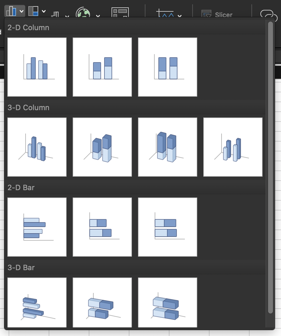
We don’t talk about specific chart types
- That you have to hunt through in Excel and reshape your data to fit it
Instead we talk about specific chart components
The Grammar of Graphics (gg) I
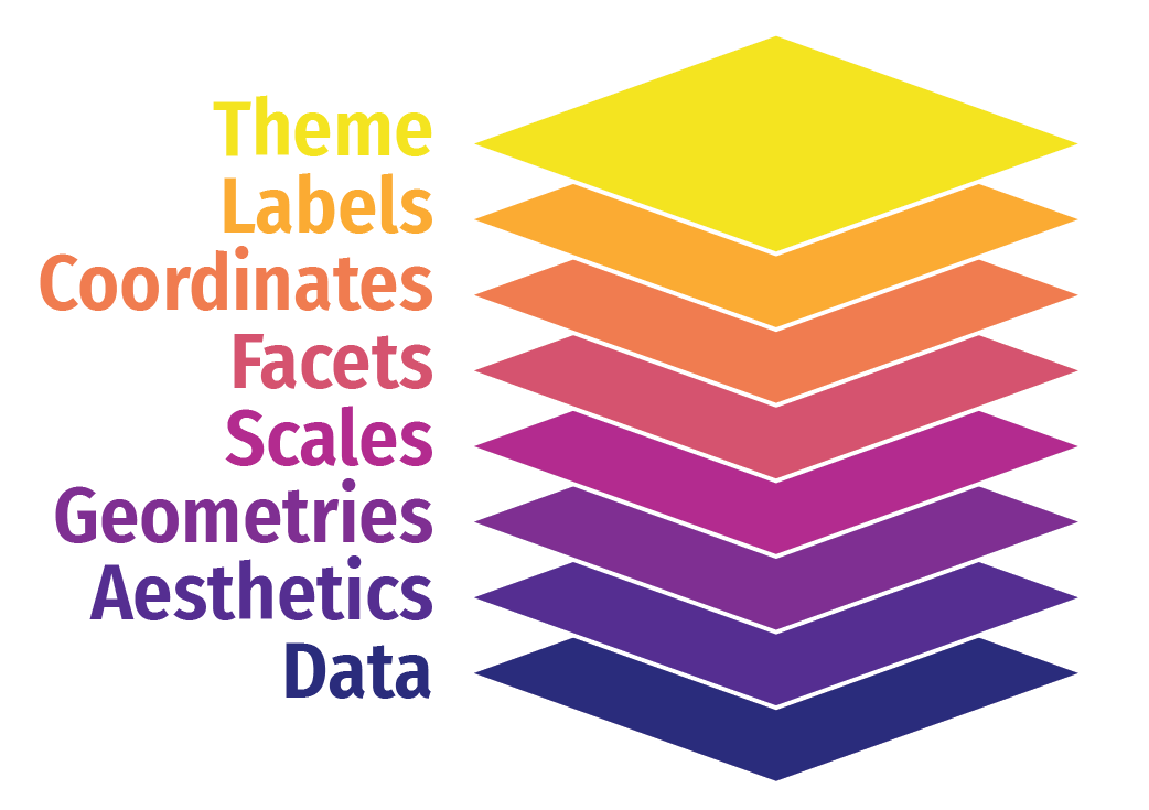
Any graphic can be built from the same components:
- Data to be drawn from
- Aesthetic mappings from data to some visual marking
- Geometric objects on the plot
- Scales define the range of values
- Coordinates to organize location
- Labels describe the scale and markings
- Facets group into subplots
- Themes style the plot elements
Not every plot needs every component, but all plots must have the first 3!
The Grammar of Graphics (gg) II
Any graphic can be built from the same components:
datato be drawn fromaesthetic mappings from data to some visual markinggeommetric objects on the plotscaledefine the range of valuescoordinates to organize locationlabelsdescribe the scale and markingsfacetgroup into subplotsthemestyle the plot elements
Not every plot needs every component, but all plots must have the first 3!
The Grammar of Graphics

The Grammar of Graphics (gg): Aesthetics I
Data
Aesthetics
+ aes()
Aesthetics map data to visual elements or parameters

The Grammar of Graphics (gg): Aesthetics II
Data
Aesthetics
+ aes()
Aesthetics map data to visual elements or parameters

The Grammar of Graphics (gg): Aesthetics IV
Data
Aesthetics
+ aes()
Aesthetics map data to visual elements or parameters

The Grammar of Graphics (gg): Geoms I
Data
Aesthetics
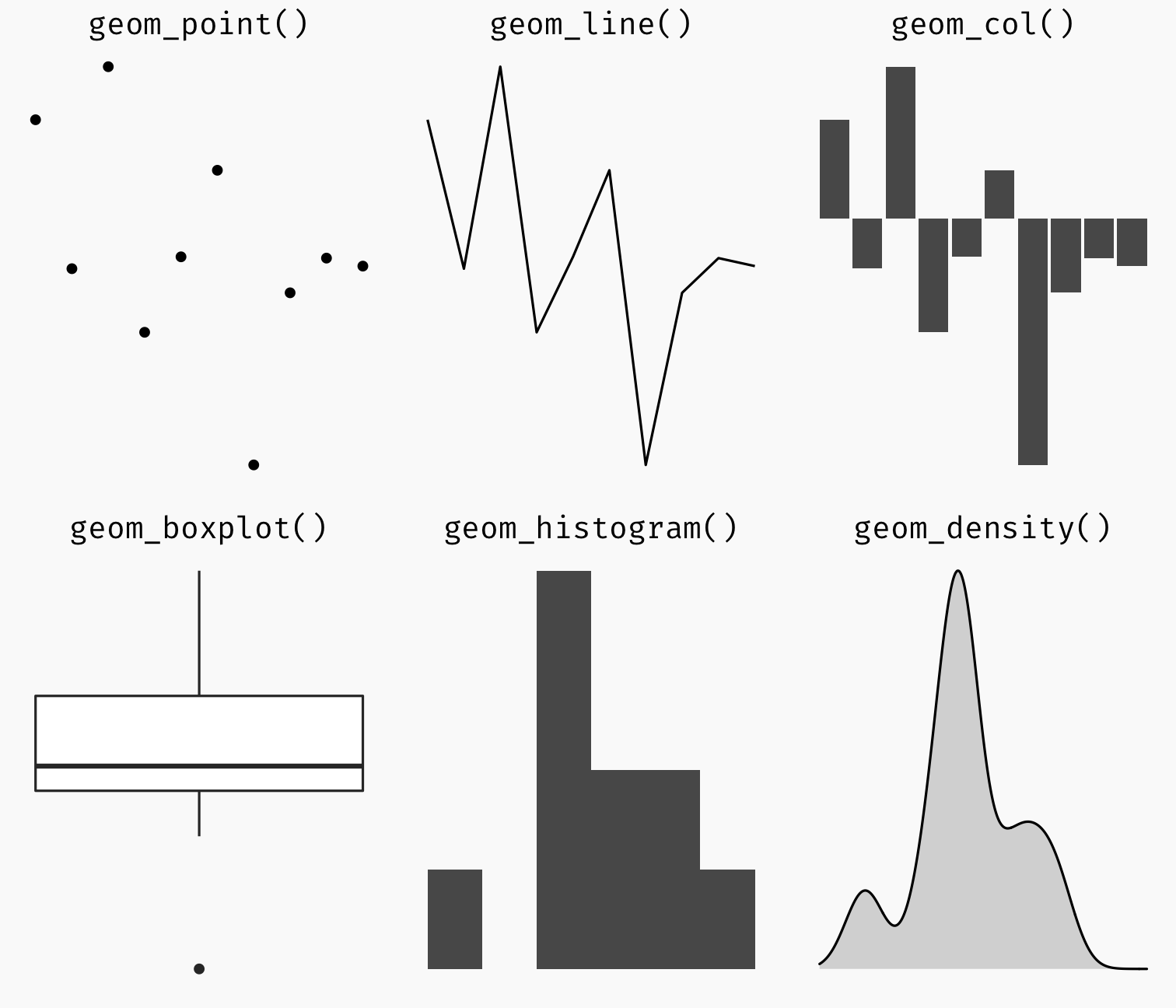
Geoms
+ geom_*()
Geometric objects displayed on the plot
The Grammar of Graphics (gg): Geoms IV
Data
Aesthetics
Geoms
+ geom_*()
Geometric objects displayed on the plot
Or just start typing geom_ in R Studio!

Let's Make a Plot!
ggplot(data = mpg)
Let's Make a Plot!
ggplot(data = mpg)+ aes(x = displ, y = hwy)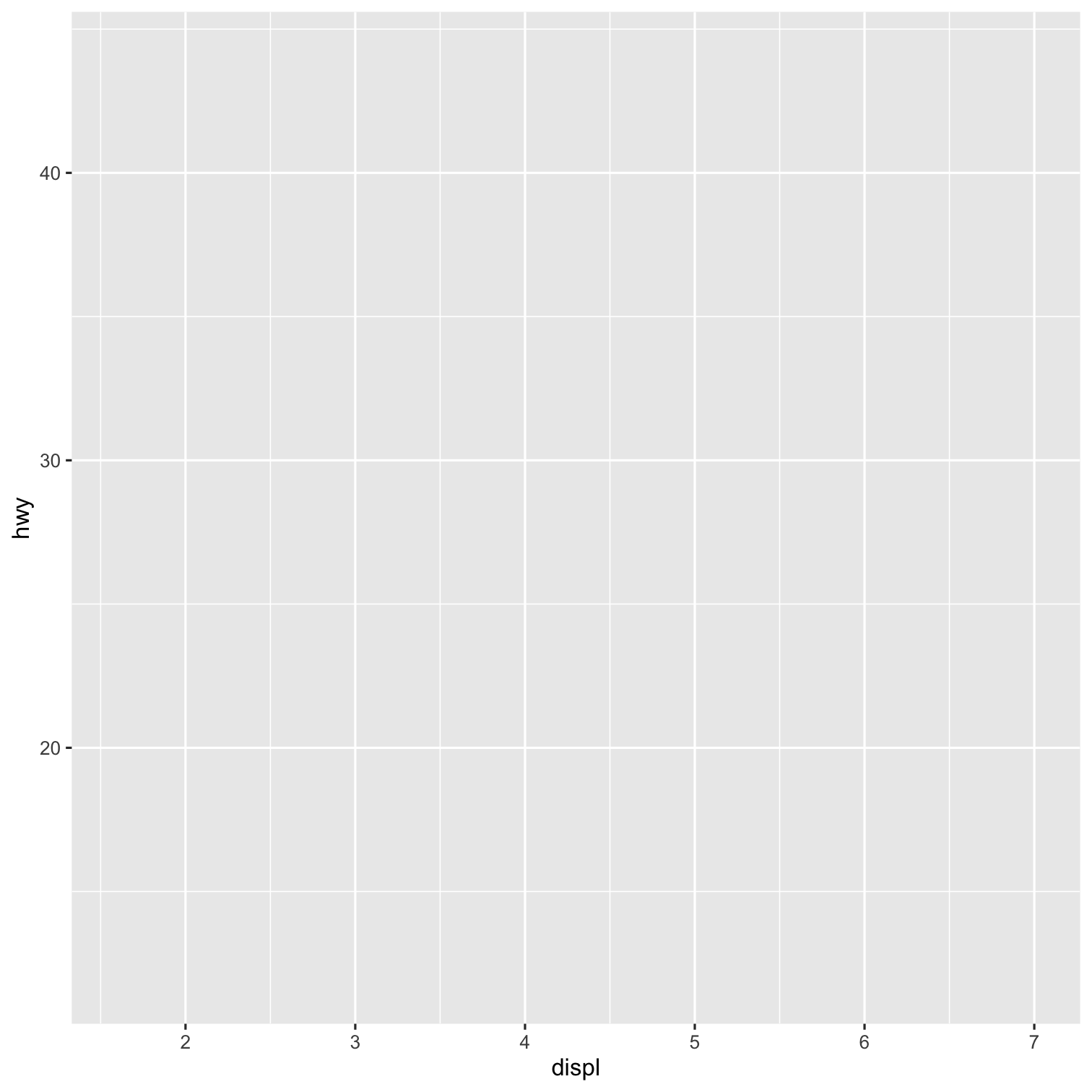
Let's Make a Plot!
ggplot(data = mpg)+ aes(x = displ, y = hwy)+ geom_point()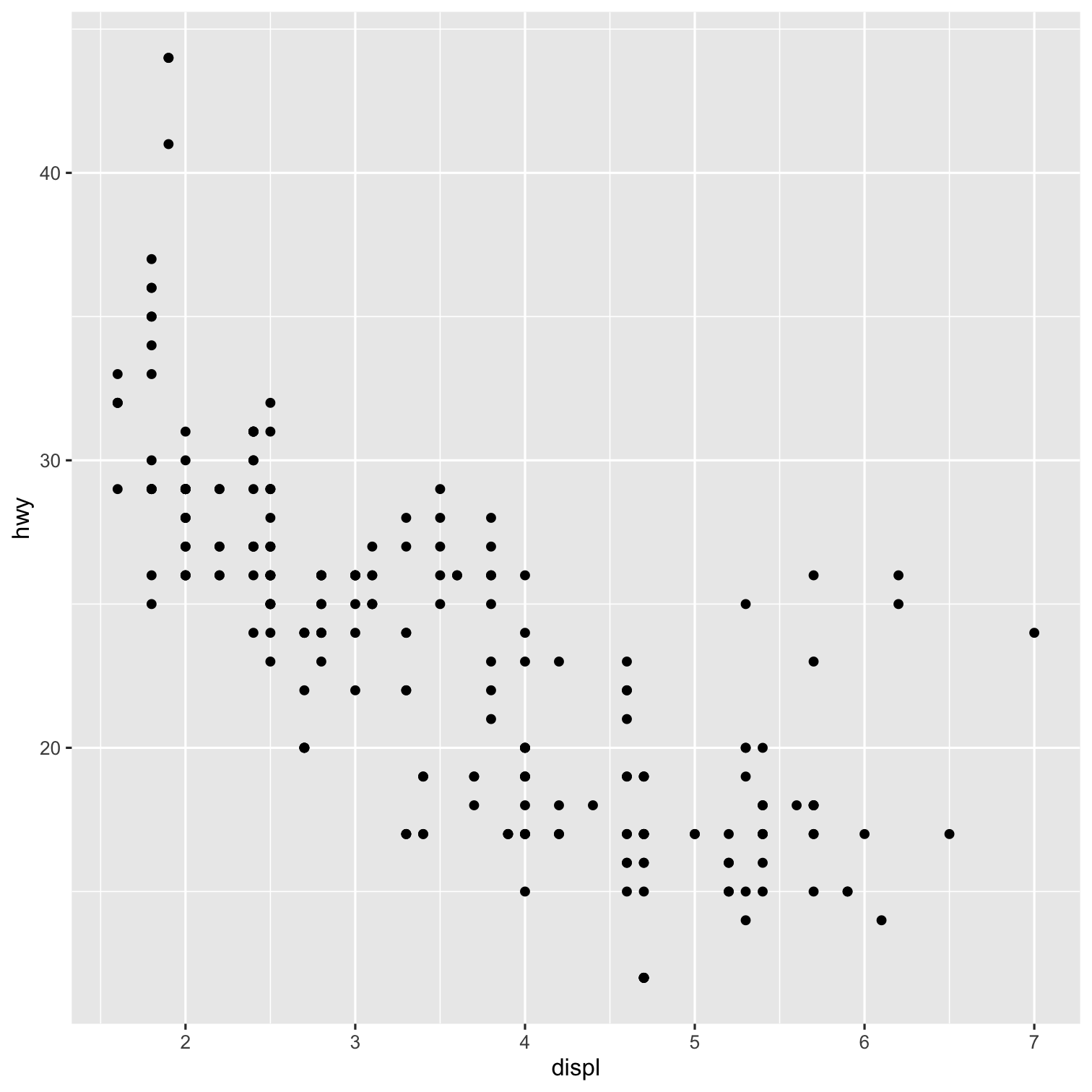
Let's Make a Plot!
ggplot(data = mpg)+ aes(x = displ, y = hwy)+ geom_point(aes(color = class))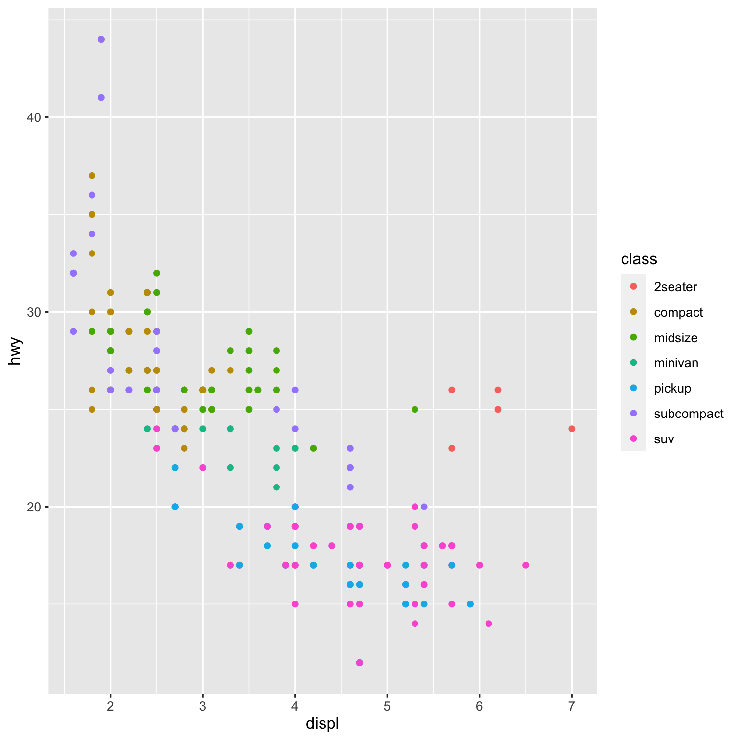
Let's Make a Plot!
ggplot(data = mpg)+ aes(x = displ, y = hwy)+ geom_point(aes(color = class))+ geom_smooth()
Change Our Plot
ggplot(data = mpg)+ aes(x = displ, y = hwy)+ geom_point(aes(color = class))+ geom_smooth()
Let's Change Our Plot
ggplot(data = mpg)+ aes(x = class, y = hwy)+ geom_boxplot()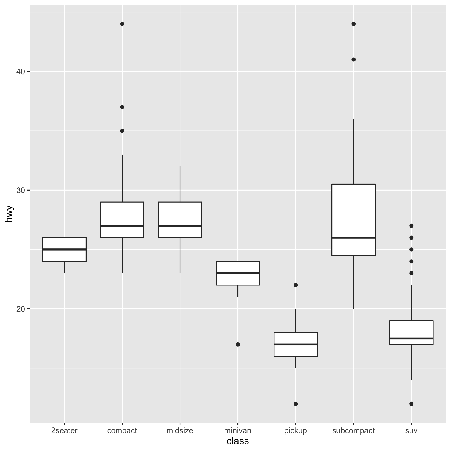
Let's Change Our Plot
ggplot(data = mpg)+ aes(x = class)+ geom_bar()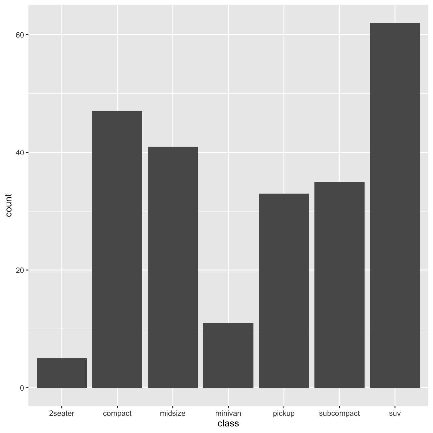
Let's Change Our Plot
ggplot(data = mpg)+ aes(x = class, fill = drv)+ geom_bar()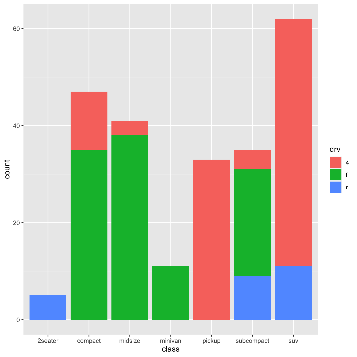
Let's Change Our Plot
ggplot(data = mpg)+ aes(x = class, fill = drv)+ geom_bar(position = "dodge")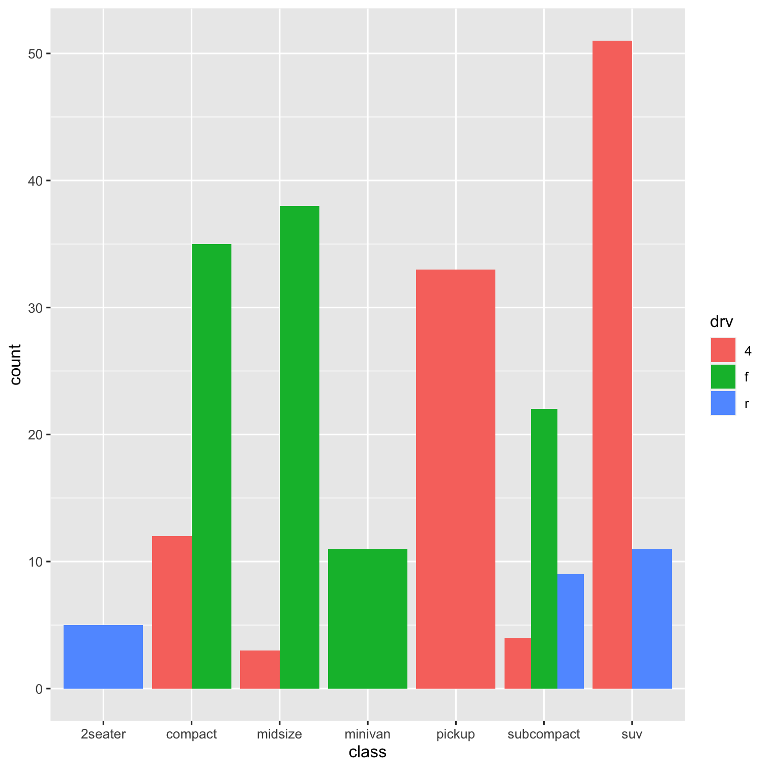
Back to the Original (and saving it)
p <- ggplot(data = mpg)+ aes(x = displ, y = hwy)+ geom_point(aes(color = class))+ geom_smooth()p # show plot
The Grammar of Graphics (gg): Facets I
Data
Aesthetics
Geoms
Facets
+ facet_wrap()
+ facet_grid()
p + facet_wrap(~year)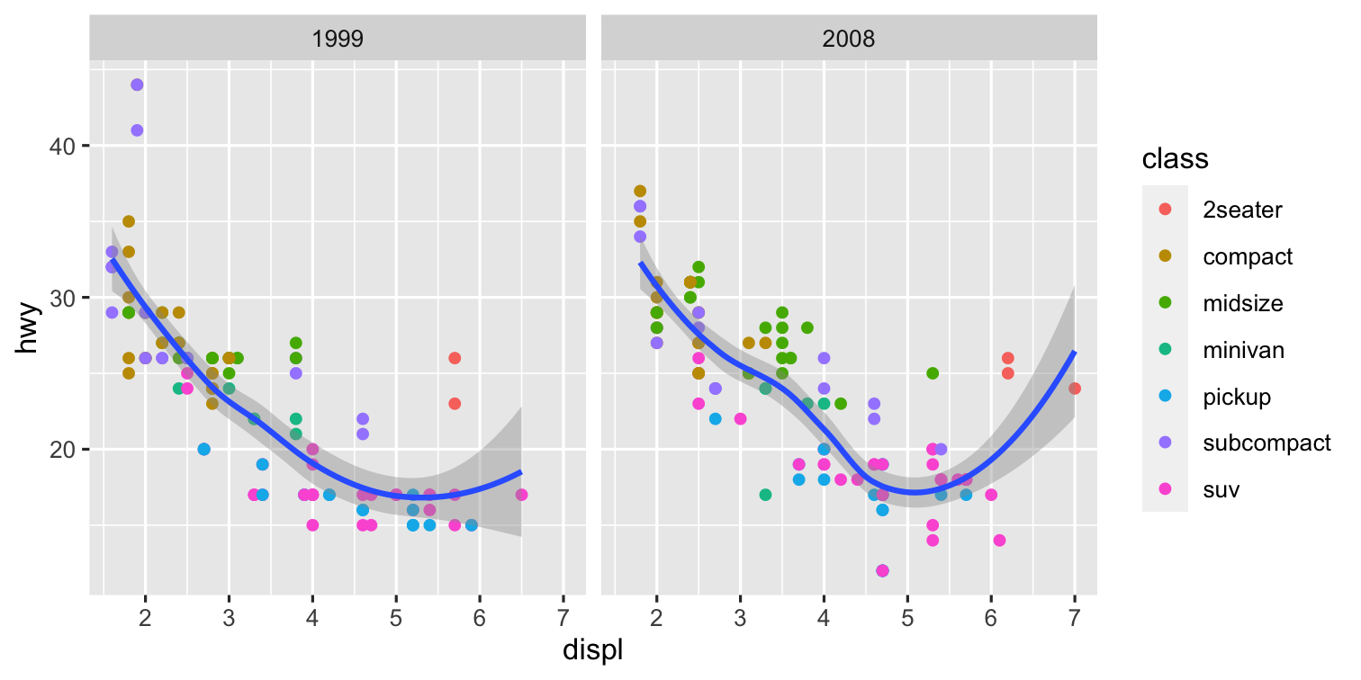
The Grammar of Graphics (gg): Facets II
Data
Aesthetics
Geoms
Facets
+ facet_wrap()
+ facet_grid()
p + facet_grid(cyl~year)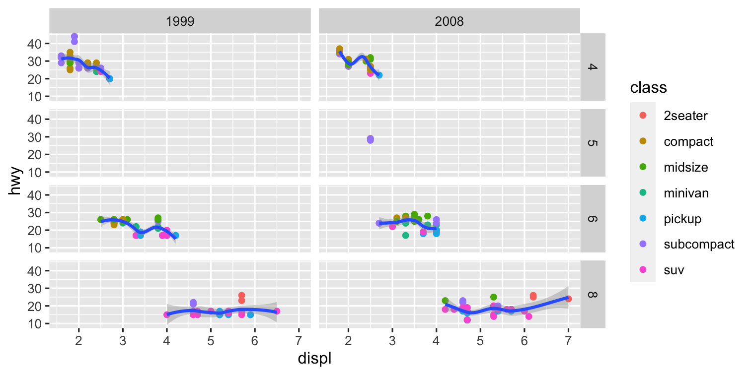
The Grammar of Graphics (gg): Labels
Data
Aesthetics
Geoms
Facets
Labels
+ labs()
p + facet_wrap(~year)+ labs(x = "Engine Displacement (Liters)", y = "Highway MPG", title = "Car Mileage and Displacement", subtitle = "More Displacement Lowers Highway MPG", caption = "Source: EPA", color = "Vehicle Class")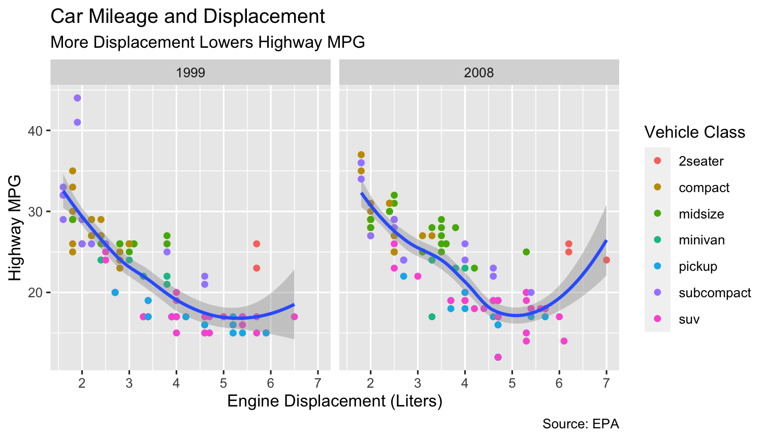
The Grammar of Graphics (gg): Scales
ggplot(data = mpg)+ aes(x = displ, y = hwy)+ geom_point(aes(color = class))+ geom_smooth()+ facet_wrap(~year)+ labs(x = "Engine Displacement (Liters)", y = "Highway MPG", title = "Car Mileage and Displacement", subtitle = "More Displacement Lowers Highway MPG", caption = "Source: EPA", color = "Vehicle Class")+ scale_color_viridis_d()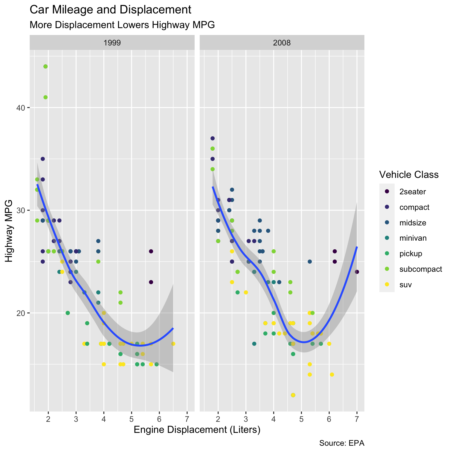
The Grammar of Graphics (gg): Themes
ggplot(data = mpg)+ aes(x = displ, y = hwy)+ geom_point(aes(color = class))+ geom_smooth()+ facet_wrap(~year)+ labs(x = "Engine Displacement (Liters)", y = "Highway MPG", title = "Car Mileage and Displacement", subtitle = "More Displacement Lowers Highway MPG", caption = "Source: EPA", color = "Vehicle Class")+ scale_color_viridis_d()+ theme_bw()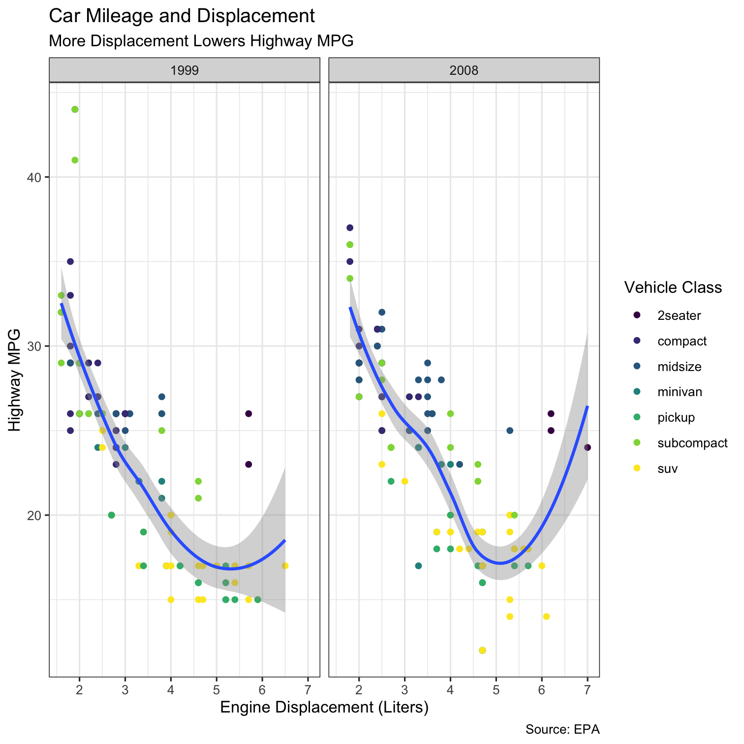
The Grammar of Graphics (gg): Themes II
ggplot(data = mpg)+ aes(x = displ, y = hwy)+ geom_point(aes(color = class))+ geom_smooth()+ facet_wrap(~year)+ labs(x = "Engine Displacement (Liters)", y = "Highway MPG", title = "Car Mileage and Displacement", subtitle = "More Displacement Lowers Highway MPG", caption = "Source: EPA", color = "Vehicle Class")+ scale_color_viridis_d()+ theme_minimal()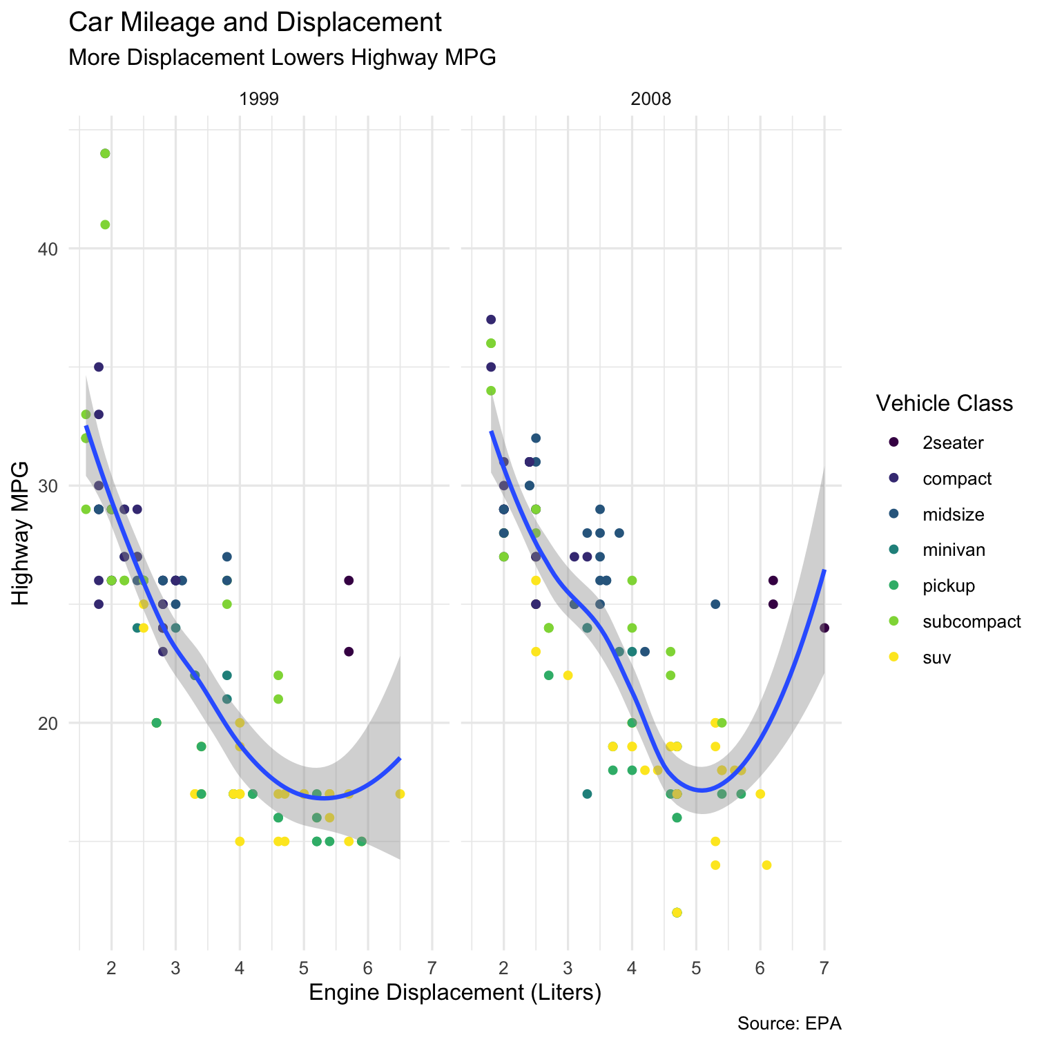
The Grammar of Graphics (gg): Themes III
ggplot(data = mpg)+ aes(x = displ, y = hwy)+ geom_point(aes(color = class))+ geom_smooth()+ facet_wrap(~year)+ labs(x = "Engine Displacement (Liters)", y = "Highway MPG", title = "Car Mileage and Displacement", subtitle = "More Displacement Lowers Highway MPG", caption = "Source: EPA", color = "Vehicle Class")+ scale_color_viridis_d()+ theme_minimal()+ theme(text = element_text(family = "Fira Sans"))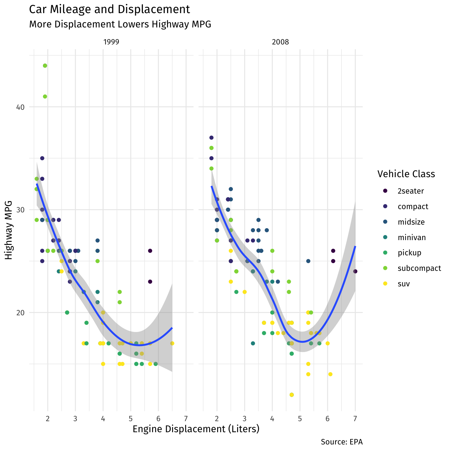
The Grammar of Graphics (gg): Themes III
ggplot(data = mpg)+ aes(x = displ, y = hwy)+ geom_point(aes(color = class))+ geom_smooth()+ facet_wrap(~year)+ labs(x = "Engine Displacement (Liters)", y = "Highway MPG", title = "Car Mileage and Displacement", subtitle = "More Displacement Lowers Highway MPG", caption = "Source: EPA", color = "Vehicle Class")+ scale_color_viridis_d()+ theme_minimal()+ theme(text = element_text(family = "Fira Sans"), legend.position="bottom")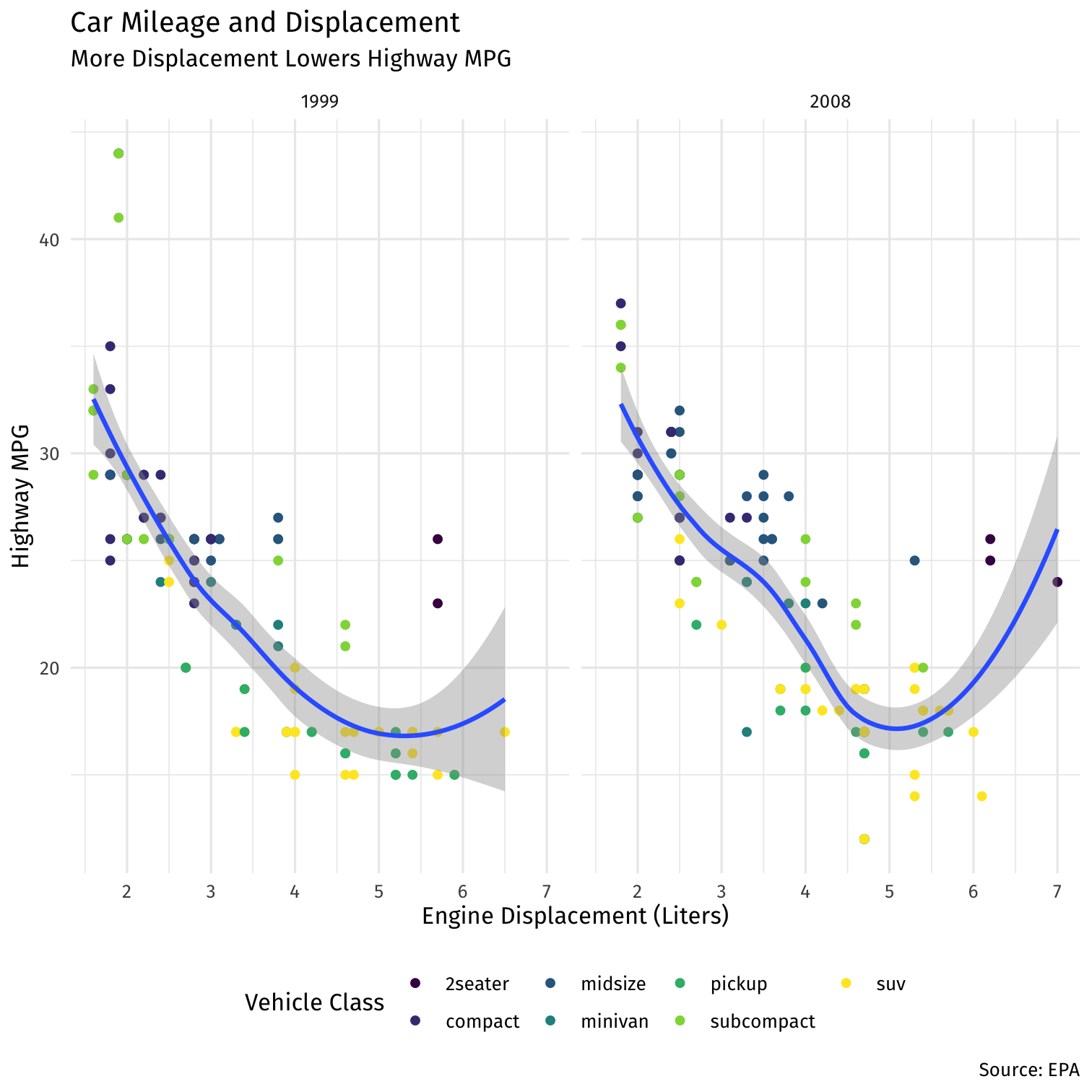
The Grammar of Graphics (gg): Themes IV
library("ggthemes")ggplot(data = mpg)+ aes(x = displ, y = hwy)+ geom_point(aes(color = class))+ geom_smooth()+ facet_wrap(~year)+ labs(x = "Engine Displacement (Liters)", y = "Highway MPG", title = "Car Mileage and Displacement", subtitle = "More Displacement Lowers Highway MPG", caption = "Source: EPA", color = "Vehicle Class")+ scale_color_viridis_d()+ theme_economist()+ theme(text = element_text(family = "Fira Sans"), legend.position="bottom")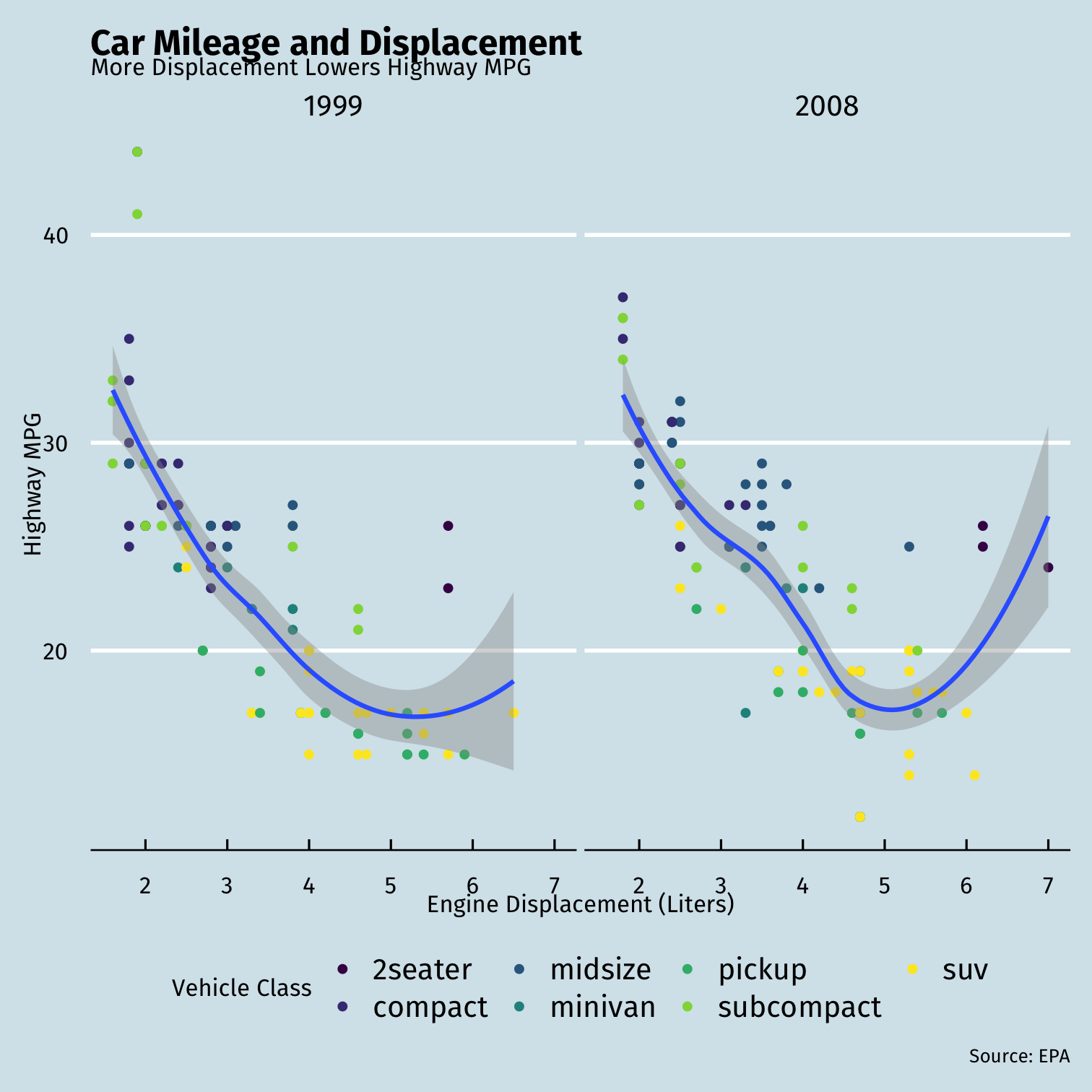
The Grammar of Graphics (gg): Themes V
library("ggthemes")ggplot(data = mpg)+ aes(x = displ, y = hwy)+ geom_point(aes(color = class))+ geom_smooth()+ facet_wrap(~year)+ labs(x = "Engine Displacement (Liters)", y = "Highway MPG", title = "Car Mileage and Displacement", subtitle = "More Displacement Lowers Highway MPG", caption = "Source: EPA", color = "Vehicle Class")+ scale_color_viridis_d()+ theme_fivethirtyeight()+ theme(text = element_text(family = "Fira Sans"), legend.position="bottom")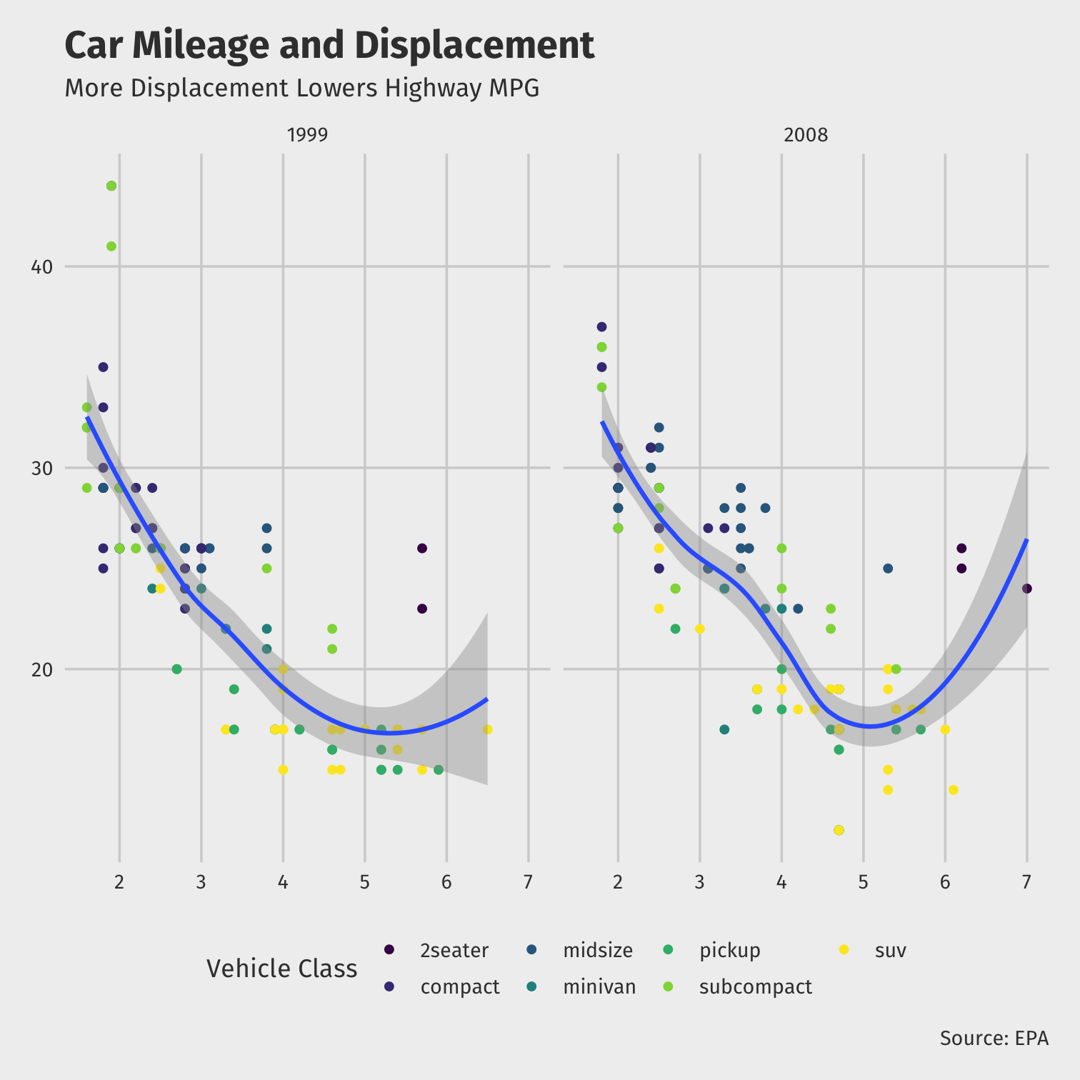
Global vs. Local Aesthetics
aes()can go in base (data) layer and/or in individualgeom()layers- All
geomswill inherit globalaesfromdatalayer unless overridden
# ALL GEOMS will map data to colorsggplot(data = mpg, aes(x = displ, y = hwy, color = class))+ geom_point()+ geom_smooth()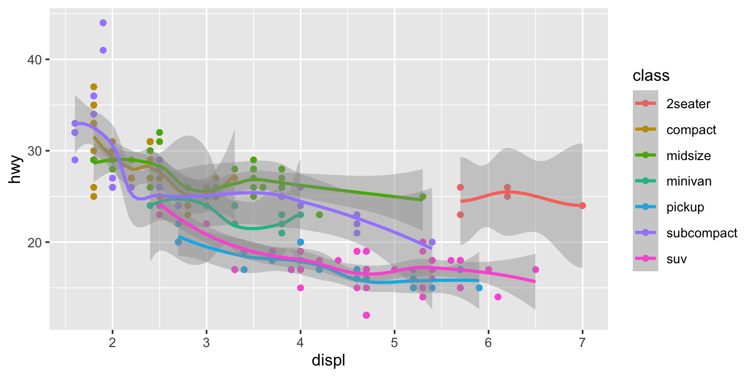
# ONLY points will map data to colorsggplot(data = mpg, aes(x = displ, y = hwy))+ geom_point(aes(color = class))+ geom_smooth()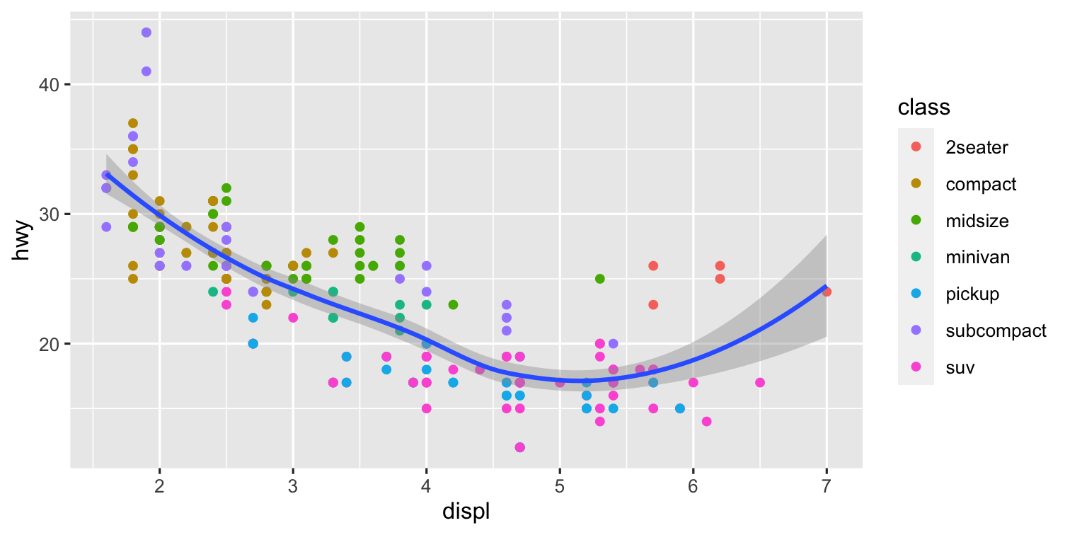
Mapped vs. Set Aesthetics
aesthetics such assizeandcolorcan be mapped from data or set to a single value- Map inside of
aes(), set outside ofaes()
# Point colors are mapped from class dataggplot(data = mpg, aes(x = displ, y = hwy))+ geom_point(aes(color = class))+ geom_smooth()
# Point colors are all set to blueggplot(data = mpg, aes(x = displ, y = hwy))+ geom_point(aes(), color = "red")+ geom_smooth(aes(), color = "blue")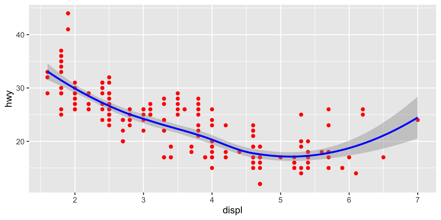
Go Crazy I
# I did some (hidden) data work before this! ggplot(data = county_full, mapping = aes(x = long, y = lat, fill = pop_dens, group = group))+ geom_polygon(color = "gray90", size = 0.05)+ coord_equal()+ scale_fill_brewer(palette="Blues", labels = c("0-10", "10-50", "50-100", "100-500", "500-1,000", "1,000-5,000", ">5,000"))+ labs(fill = "Population per\nsquare mile") + theme_map() + guides(fill = guide_legend(nrow = 1)) + theme(legend.position = "bottom")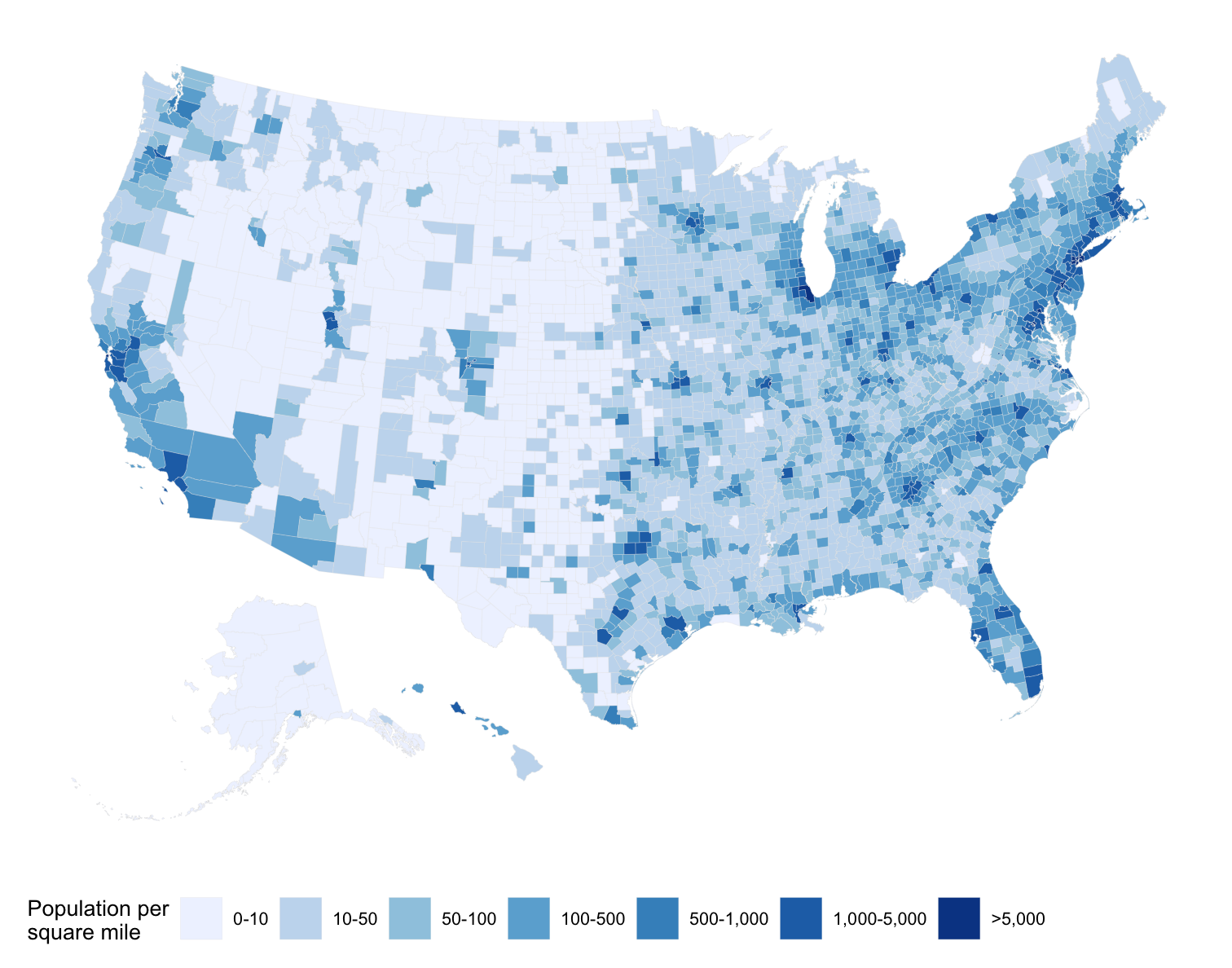
Go Crazy II
library("gapminder")library("gganimate")ggplot(gapminder) + aes(x = gdpPercap, y = lifeExp, size = pop, color = country) + geom_point() + guides(color = FALSE, size = FALSE) + scale_x_log10( breaks = c(10^3, 10^4, 10^5), labels = c("$1k", "$10k", "$100k")) + scale_color_manual(values = gapminder::country_colors) + scale_size(range = c(0.5, 12)) + labs( x = "GDP per capita", y = "Life Expectancy", caption = "Source: Hans Rosling's gapminder.org") + theme_minimal(14, base_family = "Fira Sans") + theme( strip.text = element_text(size = 16, face = "bold"), panel.border = element_rect(fill = NA, color = "grey40"), panel.grid.minor = element_blank())+ transition_states(year, 1, 0)+ ggtitle("Income and Life Expectancy - {closest_state}")
Data Visualization and Graphic Design Principles
We will return to various graphics as we cover descriptive statistics and regression
I hope to cover some basic principles of good graphic design for figures and plots
- If not in class, I will make a page on the website, and/or a video
Remember:

Less is More
"Shoot me"

Less is More
"Shoot me"
Less is More:
Try to Show One Trend Really Clearly

New York Times: "How Stable Are Democracies? ‘Warning Signs Are Flashing Red’", Nov 29, 2016
