Experiments
- An experiment is any procedure that can (in principle) be repeated infinitely and has a well-defined set of outcomes
Example: flip a coin 10 times
Random Variables
A random variable (RV) takes on values that are unknown in advance, but determined by an experiment
A numerical summary of a random outcome
Example: the number of heads from 10 coin flips
Discrete Random Variables
- A discrete random variable: takes on a finite/countable set of possible values
Example: Let X be the number of times your computer crashes this semester1, xi∈{0,1,2,3,4}

1 Please, back up your files!
Discrete Random Variables: pdf Graph
crashes<-tibble(number = c(0,1,2,3,4), prob = c(0.80, 0.10, 0.06, 0.03, 0.01))ggplot(data = crashes)+ aes(x = number, y = prob)+ geom_col(fill="#0072B2")+ labs(x = "Number of Crashes", y = "Probability")+ theme_classic(base_family = "Fira Sans Condensed", base_size=20)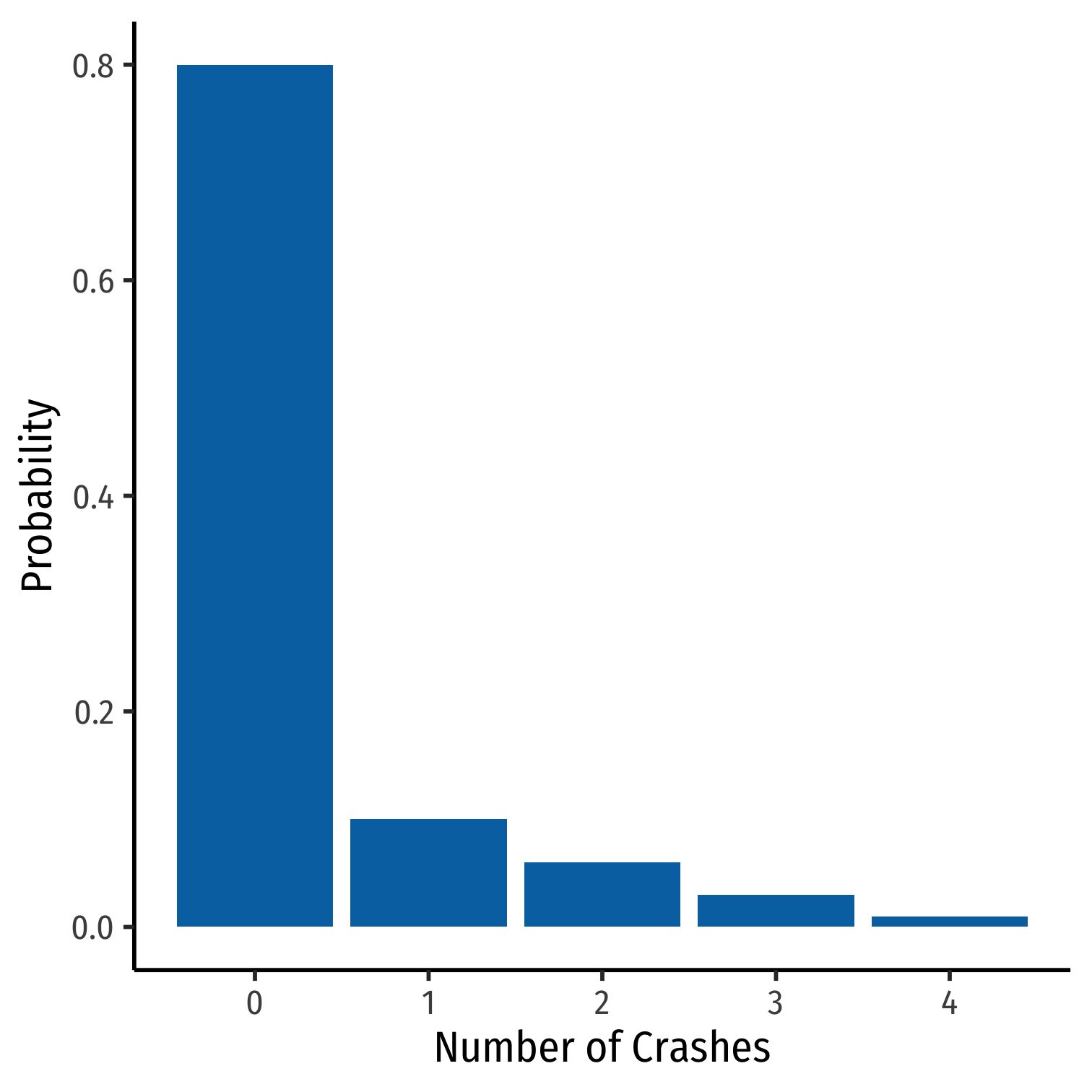
Discrete Random Variables: cdf Graph
crashes<-crashes %>% mutate(cum_prob = cumsum(prob))crashes## # A tibble: 5 × 3## number prob cum_prob## <dbl> <dbl> <dbl>## 1 0 0.8 0.8 ## 2 1 0.1 0.9 ## 3 2 0.06 0.96## 4 3 0.03 0.99## 5 4 0.01 1ggplot(data = crashes)+ aes(x = number, y = cum_prob)+ geom_col(fill="#0072B2")+ labs(x = "Number of Crashes", y = "Probability")+ theme_classic(base_family = "Fira Sans Condensed", base_size=20)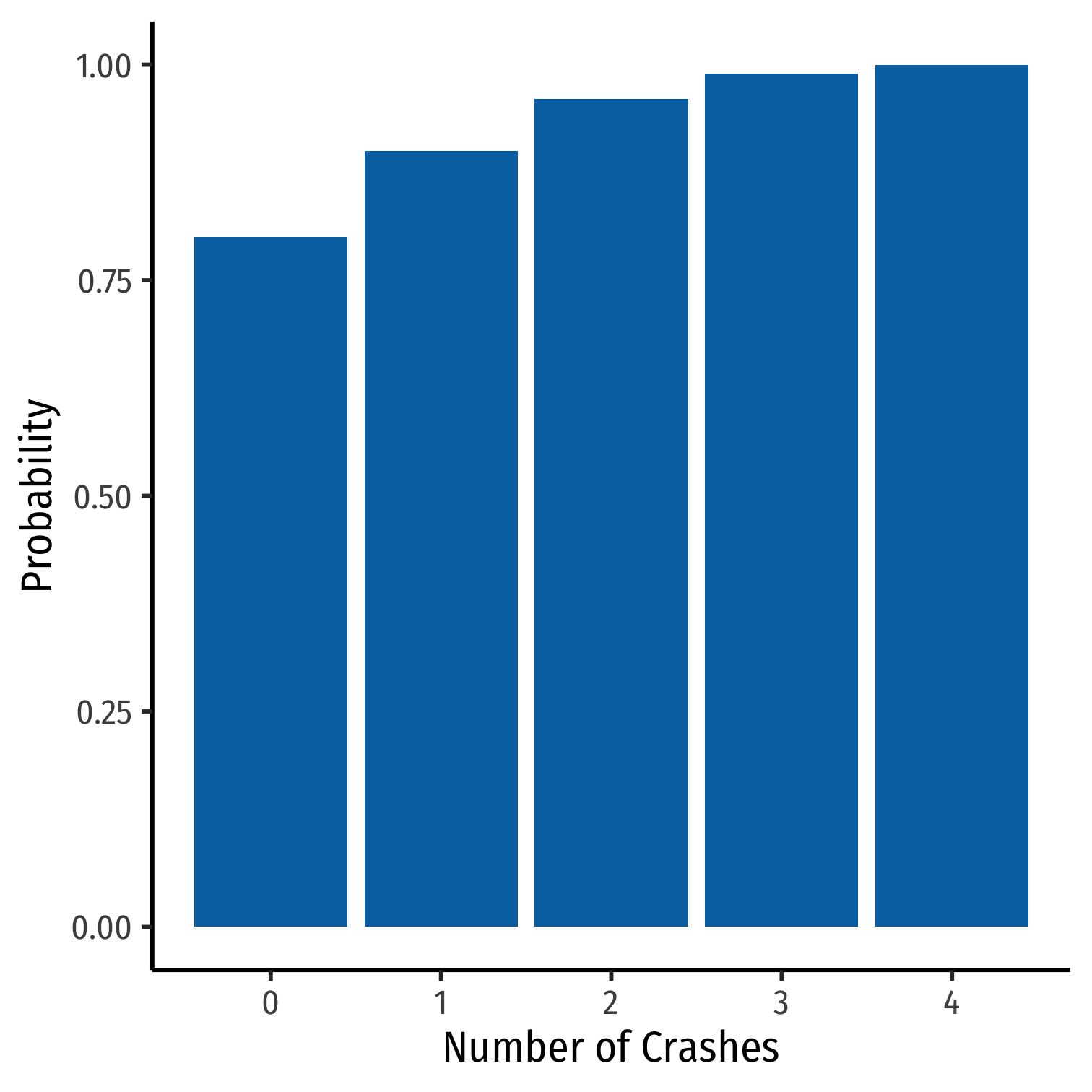
Continuous Random Variables
Continuous random variables can take on an uncountable (infinite) number of values
So many values that the probability of any specific value is infinitely small: P(X=xi)→0
Instead, we focus on a range of values it might take on

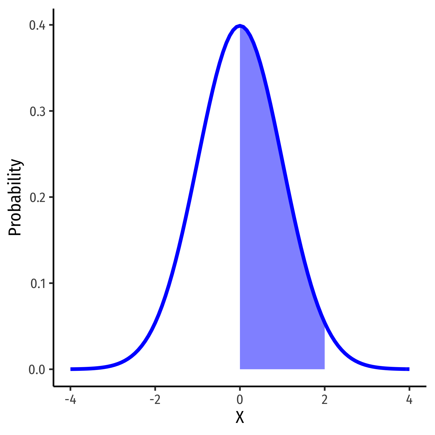
Continuous Random Variables: pdf I
Probability density function (pdf) of a continuous variable represents the probability between two values as the area under a curve
The total area under the curve is 1
Since P(a)=0 and P(b)=0, P(a<X<b)=P(a≤X≤b)
Example: P(0≤X≤2)
- See today's class notes for how to graph math/stats functions in
ggplot!
Continuous Random Variables: pdf II
- FYI using calculus:
P(a≤X≤b)=∫baf(x)dx
- Complicated: software or (old fashioned!) probability tables to calculate

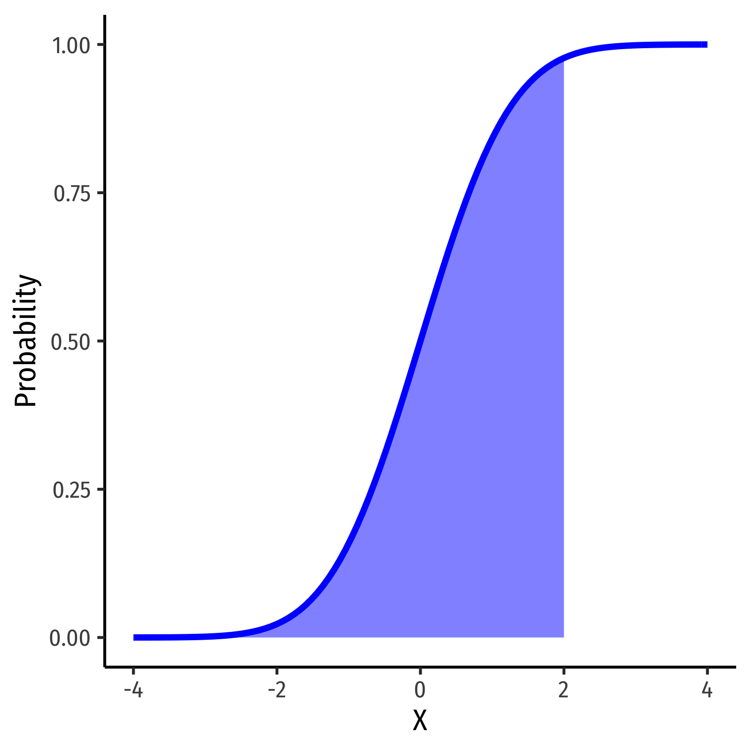
Continuous Random Variables: cdf I
- The cumulative density function (cdf) describes the area under the pdf for all values less than or equal to (i.e. to the left of) a given value, k
P(X≤k)
Example: P(X≤2)
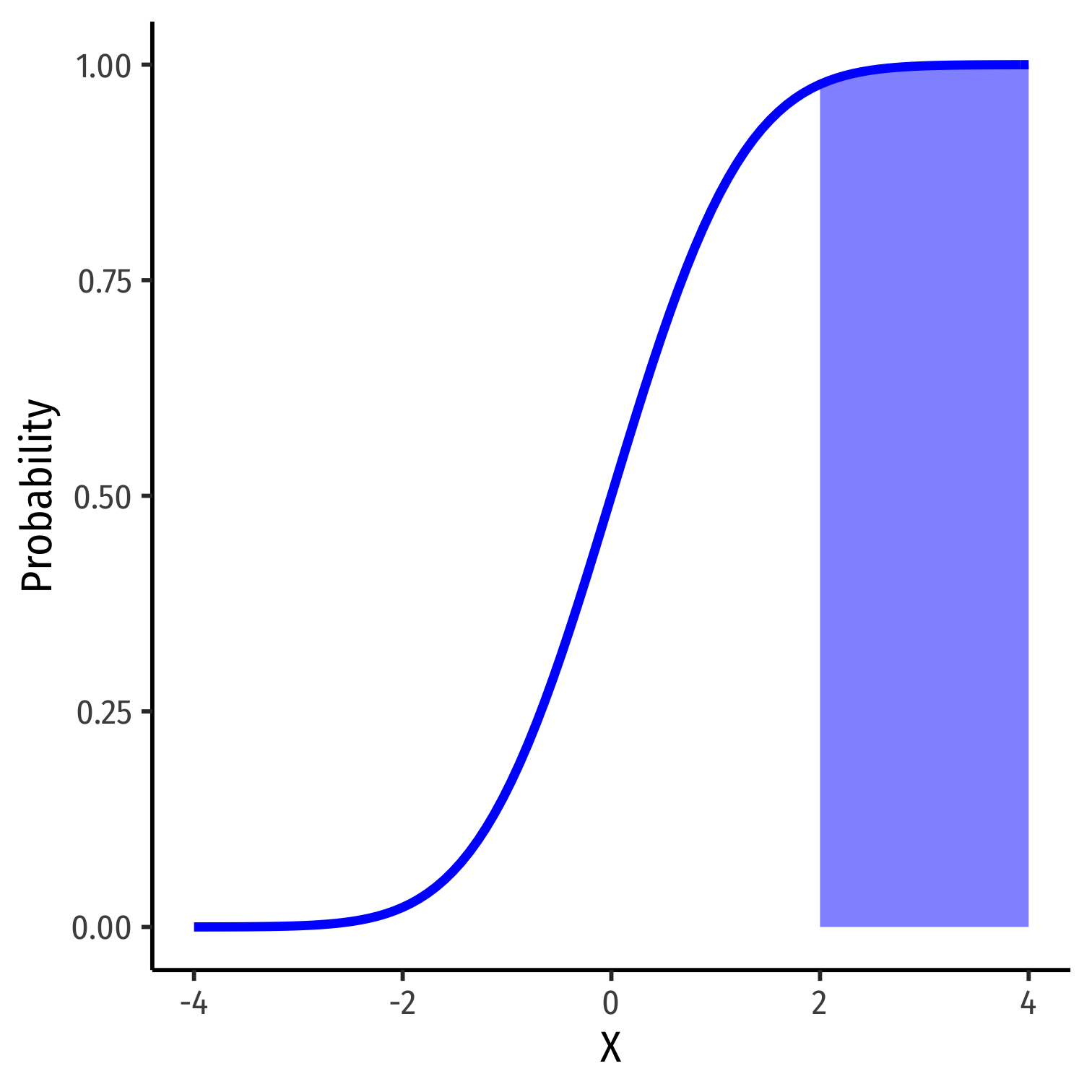
Continuous Random Variables: cdf II
- Note: to find the probability of values greater than or equal to (to the right of) a given value k:
P(X≥k)=1−P(X≤k)
Example: P(X≥2)=1−P(X≤2)
P(X≥2)= area under the curve to the right of 2
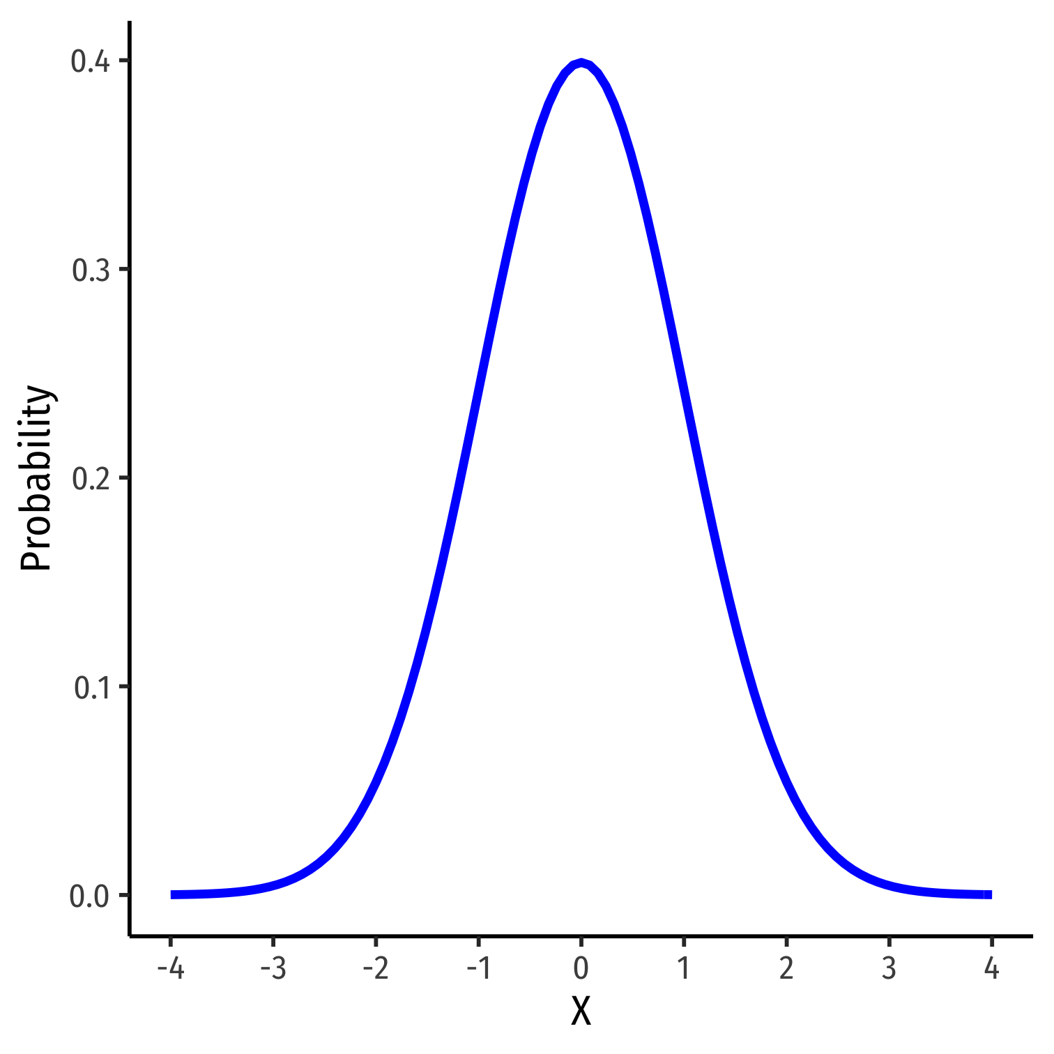
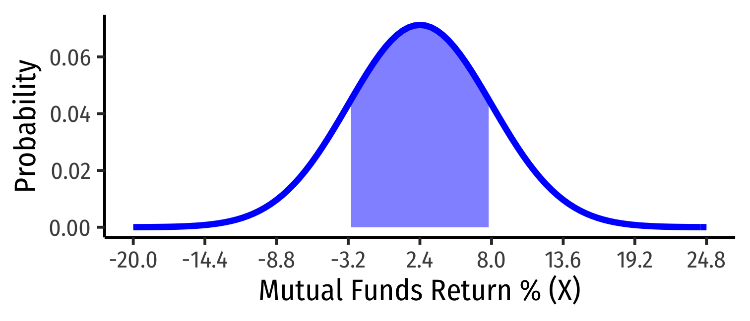
The Normal Distribution I
- The Gaussian or normal distribution is the most useful type of probability distribution
X∼N(μ,σ)
- Continuous, symmetric, unimodal, with mean μ and standard deviation σ

The Normal Distribution II
FYI: The pdf of X∼N(μ,σ) is P(X=k)=1√2πσ2e−12((k−μ)σ)2
Do not try and learn this, we have software and (previously tables) to calculate pdfs and cdfs

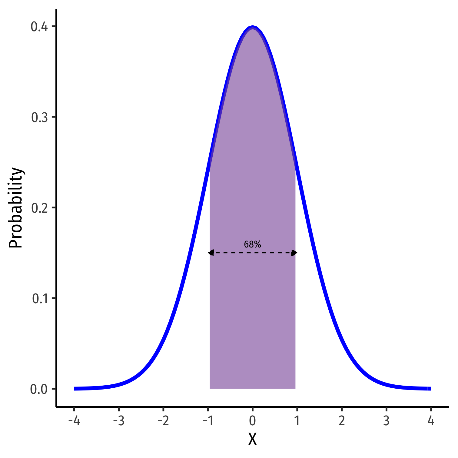
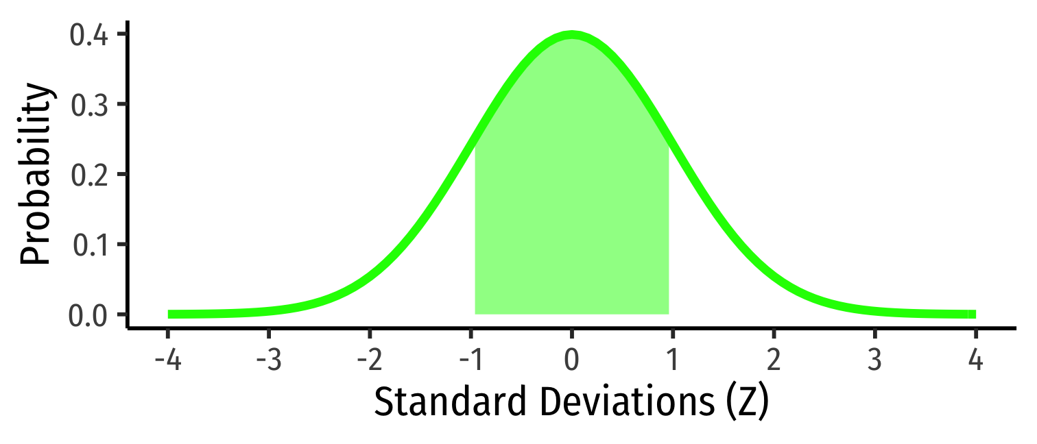
The 68-95-99.7 Rule
- 68-95-99.7% empirical rule: for a normal distribution:
The 68-95-99.7 Rule
68-95-99.7% empirical rule: for a normal distribution:
P(μ−1σ≤X≤μ+1σ)≈ 68%
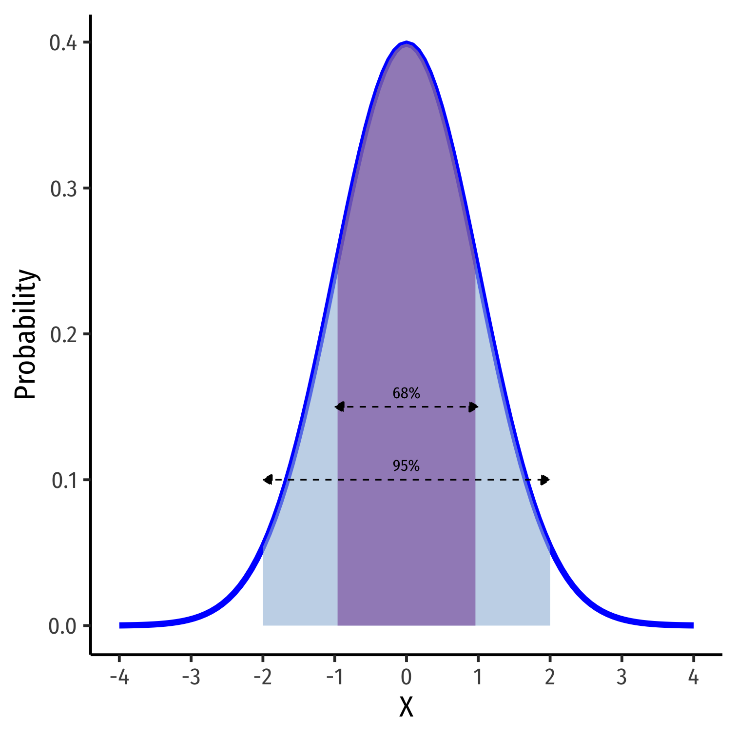
The 68-95-99.7 Rule
68-95-99.7% empirical rule: for a normal distribution:
P(μ−1σ≤X≤μ+1σ)≈ 68%
P(μ−2σ≤X≤μ+2σ)≈ 95%
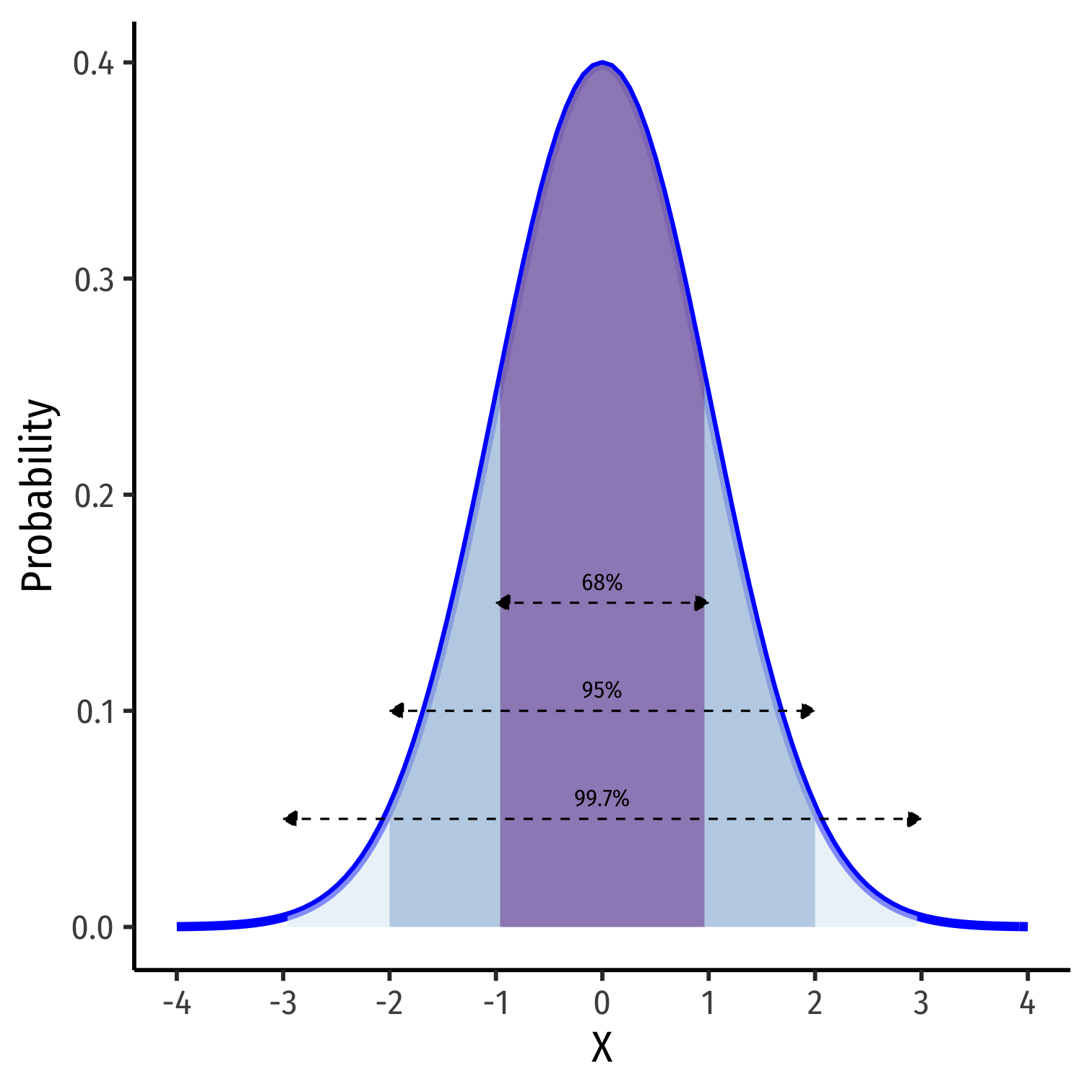
The 68-95-99.7 Rule
68-95-99.7% empirical rule: for a normal distribution:
P(μ−1σ≤X≤μ+1σ)≈ 68%
P(μ−2σ≤X≤μ+2σ)≈ 95%
P(μ−3σ≤X≤μ+3σ)≈ 99.7%
68/95/99.7% of observations fall within 1/2/3 standard deviations of the mean
The Standard Normal Distribution
- The standard normal distribution (often referred to as Z) has mean 0 and standard deviation 1
Z∼N(0,1)

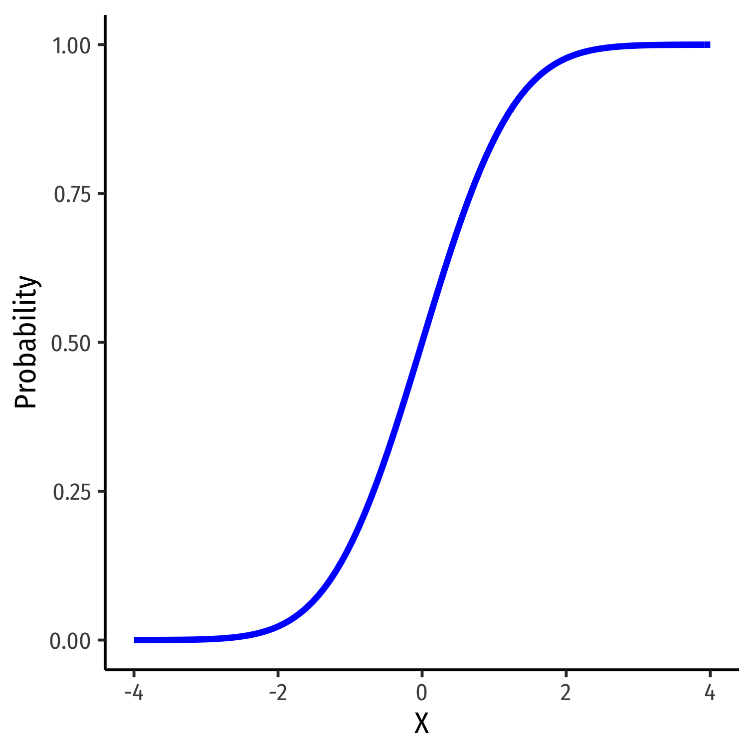
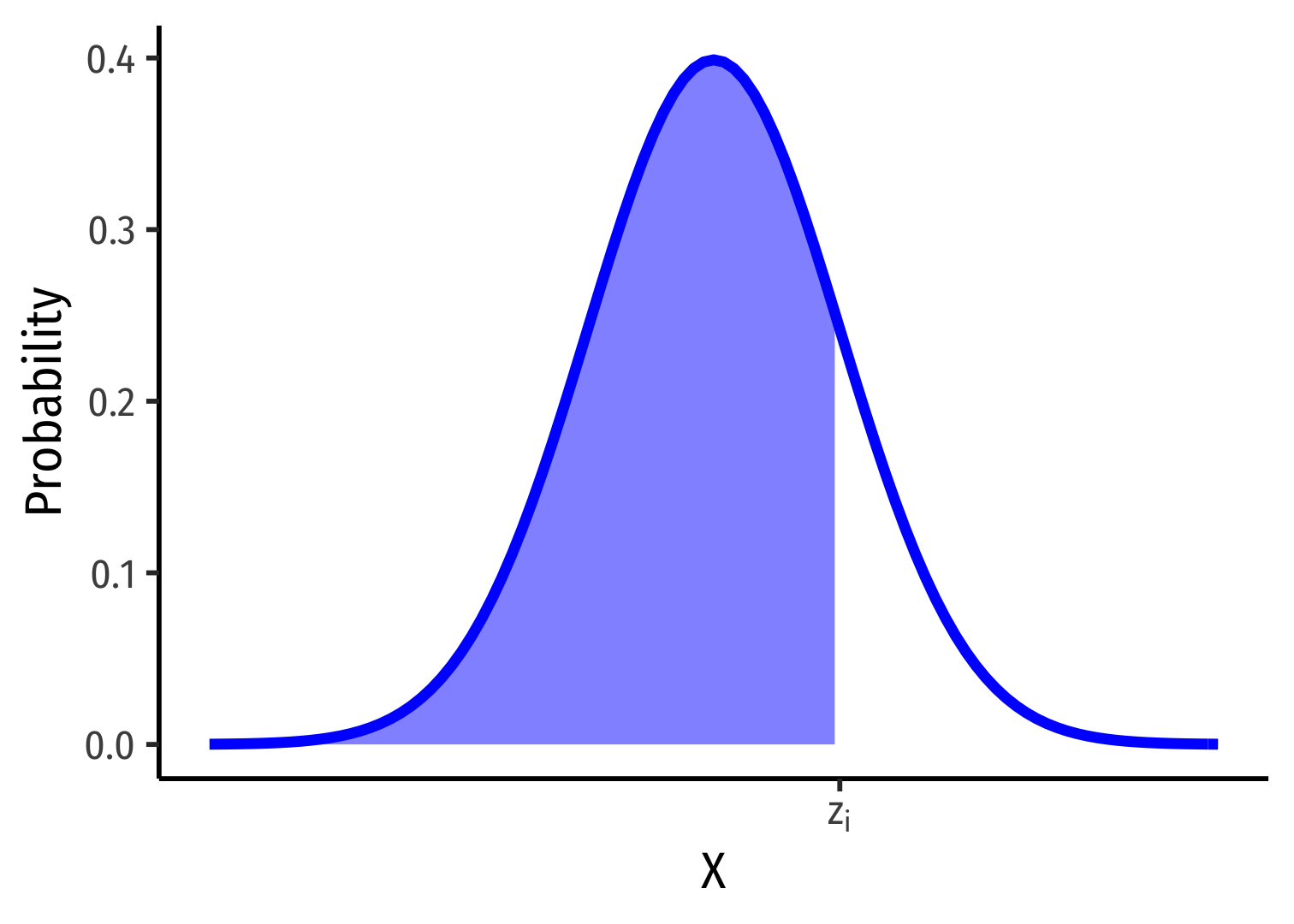
The Standard Normal cdf
- The standard normal cdf
Φ(k)=P(Z≤k)
Standardizing Variables
- We can take any normal distribution (for any μ,σ) and standardize it to the standard normal distribution by taking the Z-score of any value, xi:
Z=xi−μσ
Subtract any value by the distribution's mean and divide by standard deviation
Z: number of standard deviations xi value is away from the mean

Standardizing Variables: From X to Z II
Finding Z-score Probabilities I
- How do we actually find the probabilities for Z−scores?
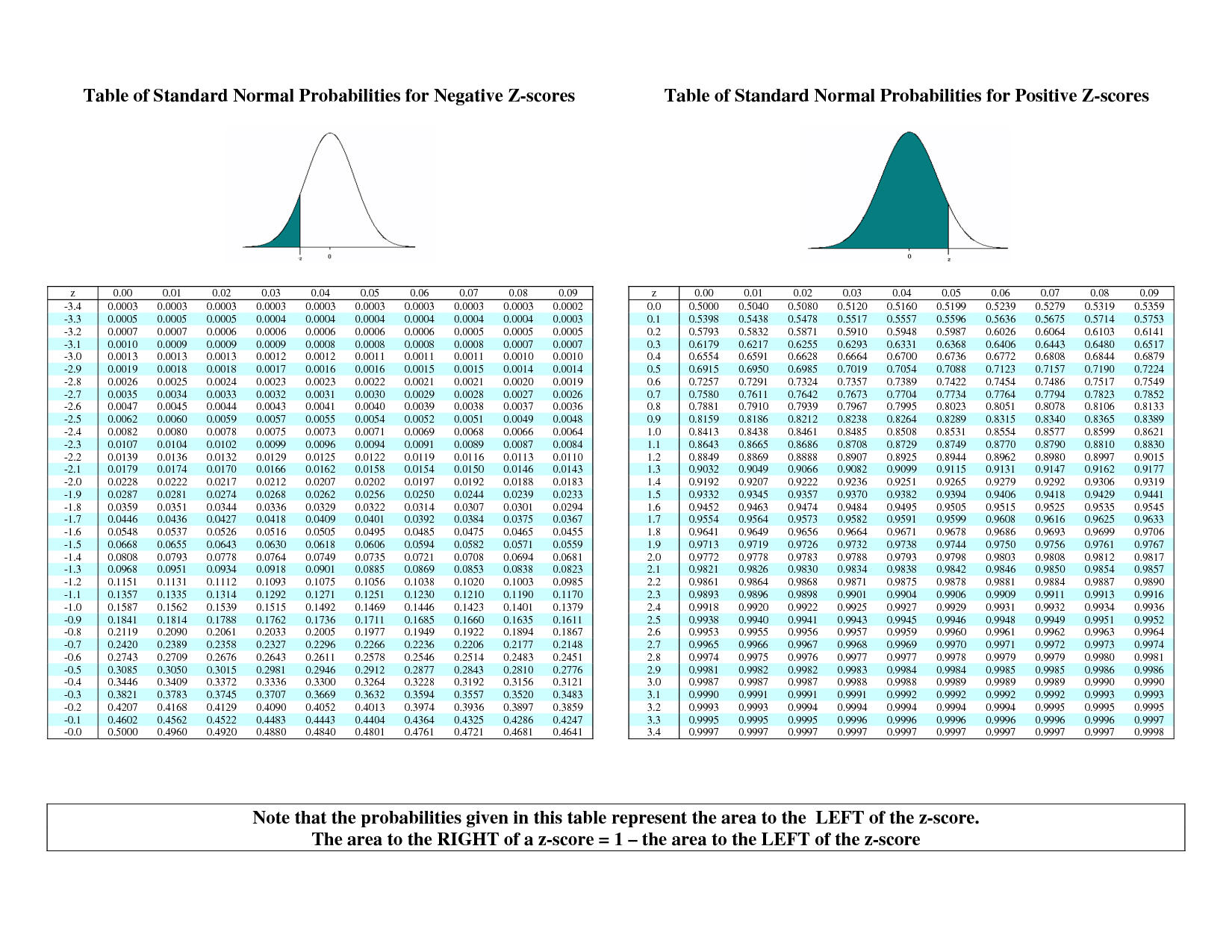
Finding Z-score Probabilities II
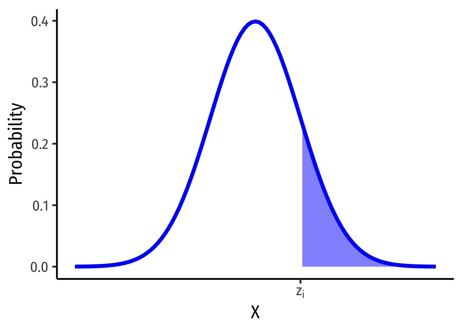
Probability to the left of zi
P(Z≤zi)=Φ(zi)⏟cdf of zi
Probability to the right of zi
P(Z≥zi)=1−Φ(zi)⏟cdf of zi
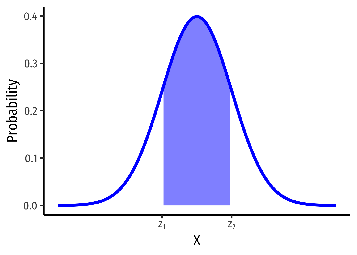
Finding Z-score Probabilities III
Probability between z1 and z2
P(z1≥Z≥z2)=Φ(z2)⏟cdf of z2−Φ(z1)⏟cdf of z1
Finding Z-score Probabilities IV
pnorm()calculatesprobabilities with anormal distribution with arguments:x =the valuemean =the meansd =the standard deviationlower.tail =TRUEif looking at area to LEFT of valueFALSEif looking at area to RIGHT of value

Finding Z-score Probabilities IV
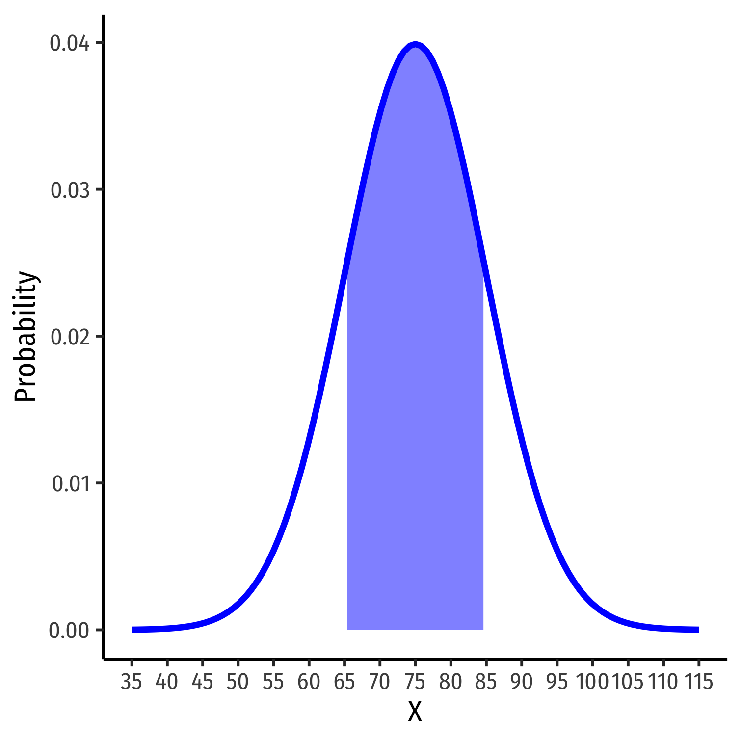
Example: Let the distribution of grades be normal, with mean 75 and standard deviation 10.
- Probability a student gets at least an 80
pnorm(80, mean = 75, sd = 10, lower.tail = FALSE) # looking to right## [1] 0.3085375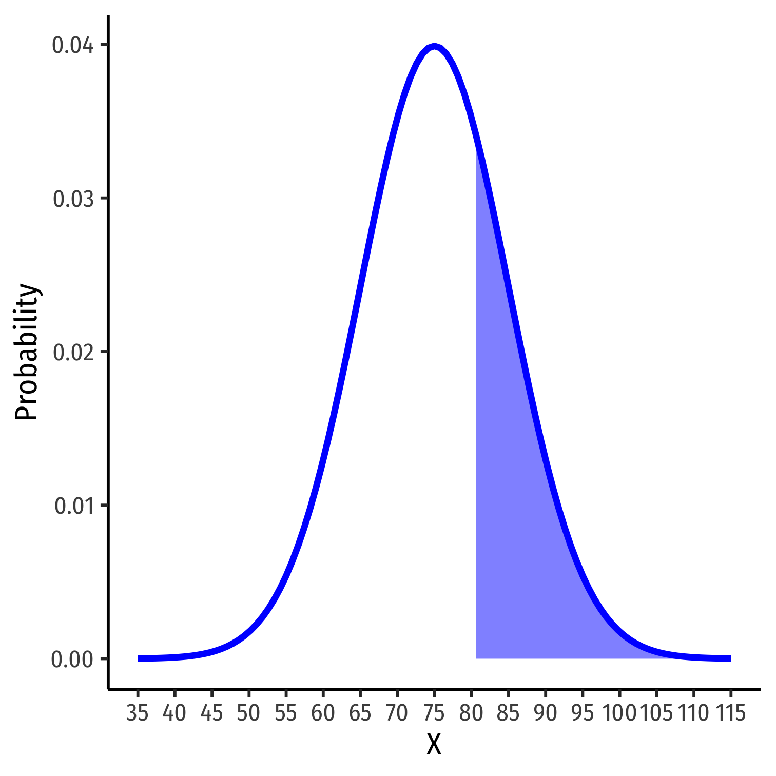
Finding Z-score Probabilities V
Example: Let the distribution of grades be normal, with mean 75 and standard deviation 10.
- Probability a student gets at most an 80
pnorm(80, mean = 75, sd = 10, lower.tail = TRUE) # looking to left## [1] 0.6914625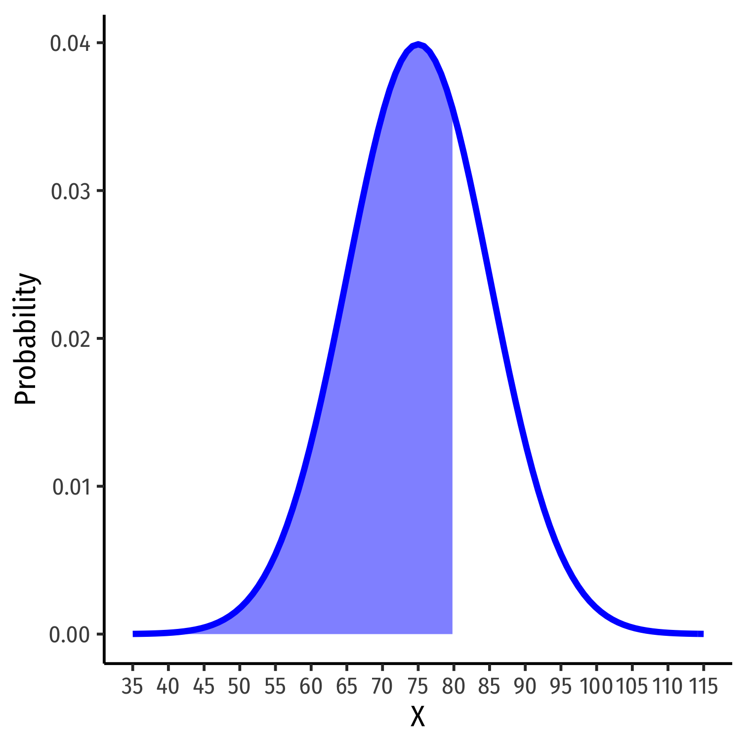
Finding Z-score Probabilities VI
Example: Let the distribution of grades be normal, with mean 75 and standard deviation 10.
- Probability a student gets between a 65 and 85
# subtract two left tails!pnorm(85, # larger number first! mean = 75, sd = 10, lower.tail = TRUE) - # looking to left, & SUBTRACT pnorm(65, # smaller number second! mean = 75, sd = 10, lower.tail = TRUE) #looking to left## [1] 0.6826895