2.5 — OLS: Precision and Diagnostics
ECON 480 • Econometrics • Fall 2021
Ryan Safner
Assistant Professor of Economics
safner@hood.edu
ryansafner/metricsF21
metricsF21.classes.ryansafner.com
The Sampling Distribution of ^β1
^β1∼N(E[^β1],σ^β1)
- Center of the distribution (last class)
- E[^β1]=β1†
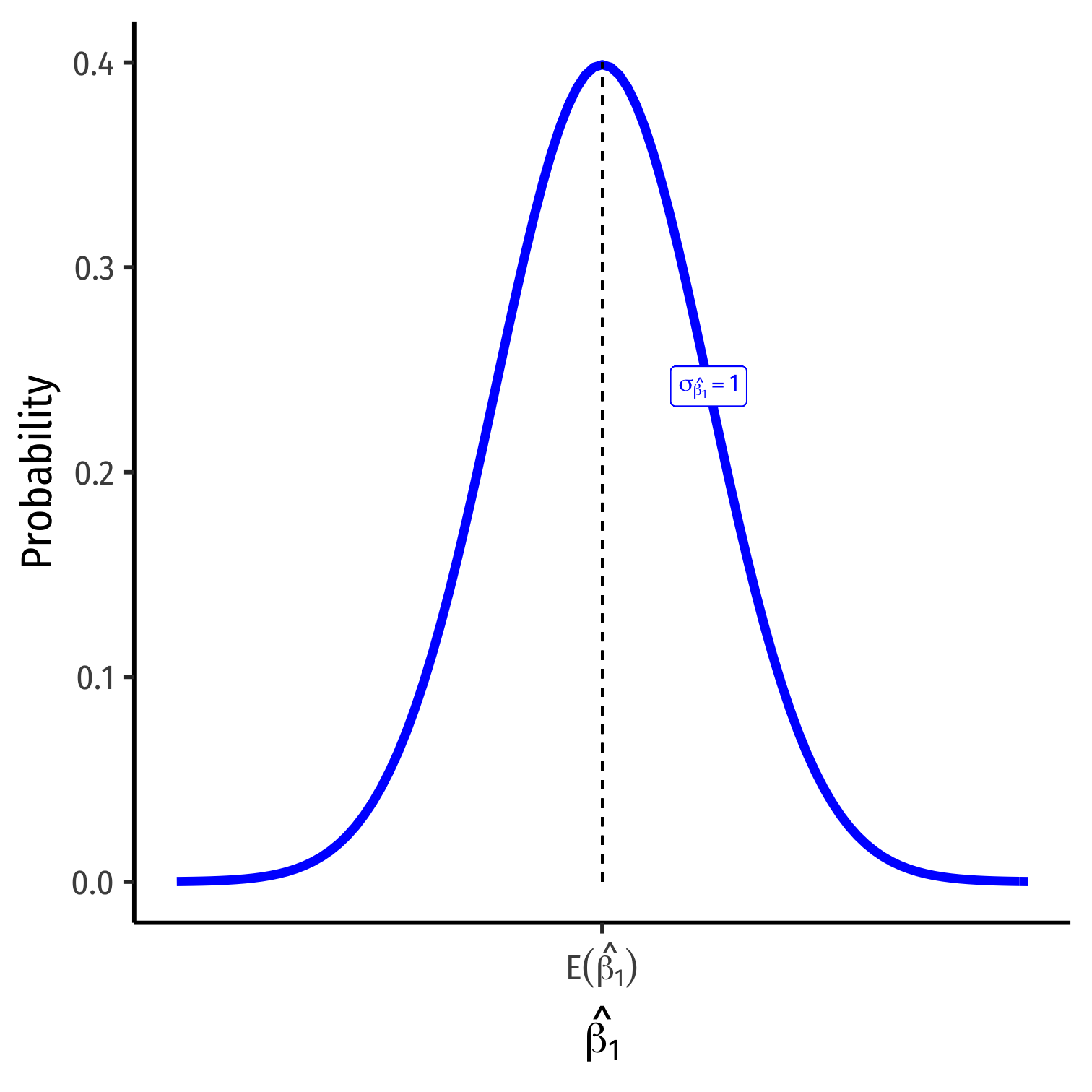
The Sampling Distribution of ^β1
^β1∼N(E[^β1],σ^β1)
Center of the distribution (last class)
- E[^β1]=β1†
How precise is our estimate? (today)
- Variance σ2^β1 or standard error‡ σ^β1
† Under the 4 assumptions about u (particularly, cor(X,u)=0).
‡ Standard “error” is the analog of standard deviation when talking about
the sampling distribution of a sample statistic (such as ˉX or ^β1).
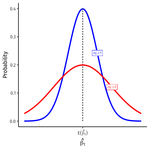
Variation in ^β1
What Affects Variation in ^β1
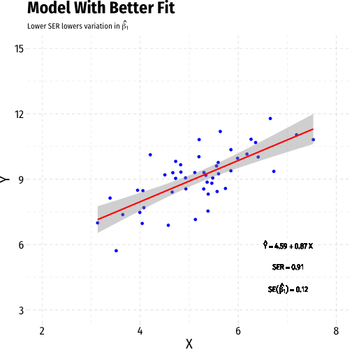
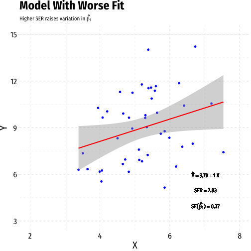
var(^β1)=(SER)2n×var(X)
se(^β1)=√var(^β1)=SER√n×sd(X)
- Variation in ^β1 is affected by 3 things:
- Goodness of fit of the model (SER)†
- Larger SER → larger var(^β1)
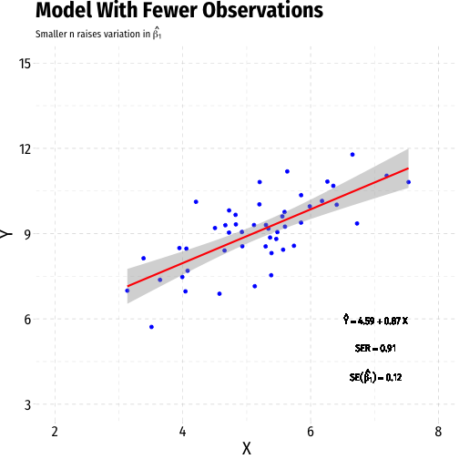
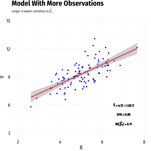
- Sample size, n
- Larger n → smaller var(^β1)
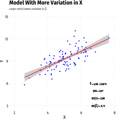
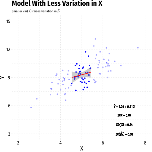
- Variance of X
- Larger var(X) → smaller var(^β1)
† Recall from last class, the Standard Error of the Regression ^σu=√∑^ui2n−2
Variation in ^β1: Goodness of Fit
Variation in ^β1: Sample Size
Variation in ^β1: Variation in X
Presenting Regression Results
Our Class Size Regression: Base R
- How can we present all of this information in a tidy way?
summary(school_reg) # get full summary## ## Call:## lm(formula = testscr ~ str, data = CASchool)## ## Residuals:## Min 1Q Median 3Q Max ## -47.727 -14.251 0.483 12.822 48.540 ## ## Coefficients:## Estimate Std. Error t value Pr(>|t|) ## (Intercept) 698.9330 9.4675 73.825 < 2e-16 ***## str -2.2798 0.4798 -4.751 2.78e-06 ***## ---## Signif. codes: 0 '***' 0.001 '**' 0.01 '*' 0.05 '.' 0.1 ' ' 1## ## Residual standard error: 18.58 on 418 degrees of freedom## Multiple R-squared: 0.05124, Adjusted R-squared: 0.04897 ## F-statistic: 22.58 on 1 and 418 DF, p-value: 2.783e-06Our Class Size Regression: Broom I

broom'stidy()function creates a tidy tibble of regression output
# load broomlibrary(broom)# tidy regression outputtidy(school_reg)## # A tibble: 2 × 5## term estimate std.error statistic p.value## <chr> <dbl> <dbl> <dbl> <dbl>## 1 (Intercept) 699. 9.47 73.8 6.57e-242## 2 str -2.28 0.480 -4.75 2.78e- 6Our Class Size Regression: Broom II
broom'sglance()gives us summary statistics about the regression
glance(school_reg)## # A tibble: 1 × 12## r.squared adj.r.squared sigma statistic p.value df logLik AIC BIC## <dbl> <dbl> <dbl> <dbl> <dbl> <dbl> <dbl> <dbl> <dbl>## 1 0.0512 0.0490 18.6 22.6 0.00000278 1 -1822. 3650. 3663.## # … with 3 more variables: deviance <dbl>, df.residual <int>, nobs <int>Presenting Regressions in a Table
Professional journals and papers often have a regression table, including:
- Estimates of ^β0 and ^β1
- Standard errors of ^β0 and ^β1 (often below, in parentheses)
- Indications of statistical significance (often with asterisks)
- Measures of regression fit: R2, SER, etc
Later: multiple rows & columns for multiple variables & models
| Test Score | |
|---|---|
| Intercept | 698.93 *** |
| (9.47) | |
| STR | -2.28 *** |
| (0.48) | |
| N | 420 |
| R-Squared | 0.05 |
| SER | 18.58 |
| *** p < 0.001; ** p < 0.01; * p < 0.05. | |
Regression Output with huxtable I
You will need to first
install.packages("huxtable")Load with
library(huxtable)Command:
huxreg()Main argument is the name of your
lmobjectDefault output is fine, but often we want to customize a bit
# install.packages("huxtable")library(huxtable)huxreg(school_reg)| (1) | |
|---|---|
| (Intercept) | 698.933 *** |
| (9.467) | |
| str | -2.280 *** |
| (0.480) | |
| N | 420 |
| R2 | 0.051 |
| logLik | -1822.250 |
| AIC | 3650.499 |
| *** p < 0.001; ** p < 0.01; * p < 0.05. | |
Regression Output with huxtable II
- Can give title to each column
"Test Score" = school_regRegression Output with huxtable II
- Can give title to each column
"Test Score" = school_reg- Can change name of coefficients from default
coefs = c("Intercept" = "(Intercept)", "STR" = "str")Regression Output with huxtable II
- Can give title to each column
"Test Score" = school_reg- Can change name of coefficients from default
coefs = c("Intercept" = "(Intercept)", "STR" = "str")- Decide what statistics to include, and rename them
statistics = c("N" = "nobs", "R-Squared" = "r.squared", "SER" = "sigma")Regression Output with huxtable II
- Can give title to each column
"Test Score" = school_reg- Can change name of coefficients from default
coefs = c("Intercept" = "(Intercept)", "STR" = "str")- Decide what statistics to include, and rename them
statistics = c("N" = "nobs", "R-Squared" = "r.squared", "SER" = "sigma")- Choose how many decimal places to round to
number_format = 2Regression Output with huxtable III
huxreg("Test Score" = school_reg, coefs = c("Intercept" = "(Intercept)", "STR" = "str"), statistics = c("N" = "nobs", "R-Squared" = "r.squared", "SER" = "sigma"), number_format = 2)Regression Output with huxtable III
huxreg("Test Score" = school_reg, coefs = c("Intercept" = "(Intercept)", "STR" = "str"), statistics = c("N" = "nobs", "R-Squared" = "r.squared", "SER" = "sigma"), number_format = 2)| Test Score | |
|---|---|
| Intercept | 698.93 *** |
| (9.47) | |
| STR | -2.28 *** |
| (0.48) | |
| N | 420 |
| R-Squared | 0.05 |
| SER | 18.58 |
| *** p < 0.001; ** p < 0.01; * p < 0.05. | |
Regression Outputs
huxtableis one package you can useI used to only use
stargazer, but as it was originally meant for STATA, it has limits and problems- A great cheetsheat by my friend Jake Russ
Diagnostics about Regression
Diagnostics: Residuals I
We often look at the residuals of a regression to get more insight about its goodness of fit and its bias
Recall
broom'saugmentcreates some useful new variables.fittedare fitted (predicted) values from model, i.e. ˆYi.residare residuals (errors) from model, i.e. ˆui
Diagnostics: Residuals II
- Often a good idea to store in a new object (so we can make some plots)
aug_reg<-augment(school_reg)aug_reg %>% head()| testscr | str | .fitted | .resid | .hat | .sigma | .cooksd | .std.resid |
|---|---|---|---|---|---|---|---|
| 691 | 17.9 | 658 | 32.7 | 0.00442 | 18.5 | 0.00689 | 1.76 |
| 661 | 21.5 | 650 | 11.3 | 0.00475 | 18.6 | 0.000893 | 0.612 |
| 644 | 18.7 | 656 | -12.7 | 0.00297 | 18.6 | 0.0007 | -0.685 |
| 648 | 17.4 | 659 | -11.7 | 0.00586 | 18.6 | 0.00117 | -0.629 |
| 641 | 18.7 | 656 | -15.5 | 0.00301 | 18.6 | 0.00105 | -0.836 |
| 606 | 21.4 | 650 | -44.6 | 0.00446 | 18.5 | 0.013 | -2.4 |
Recap: Assumptions about Errors
- We make 4 critical assumptions about u:
The expected value of the residuals is 0 E[u]=0
The variance of the residuals over X is constant: var(u|X)=σ2u
Errors are not correlated across observations: cor(ui,uj)=0∀i≠j
There is no correlation between X and the error term: cor(X,u)=0 or E[u|X]=0

Assumptions 1 and 2: Errors are i.i.d.
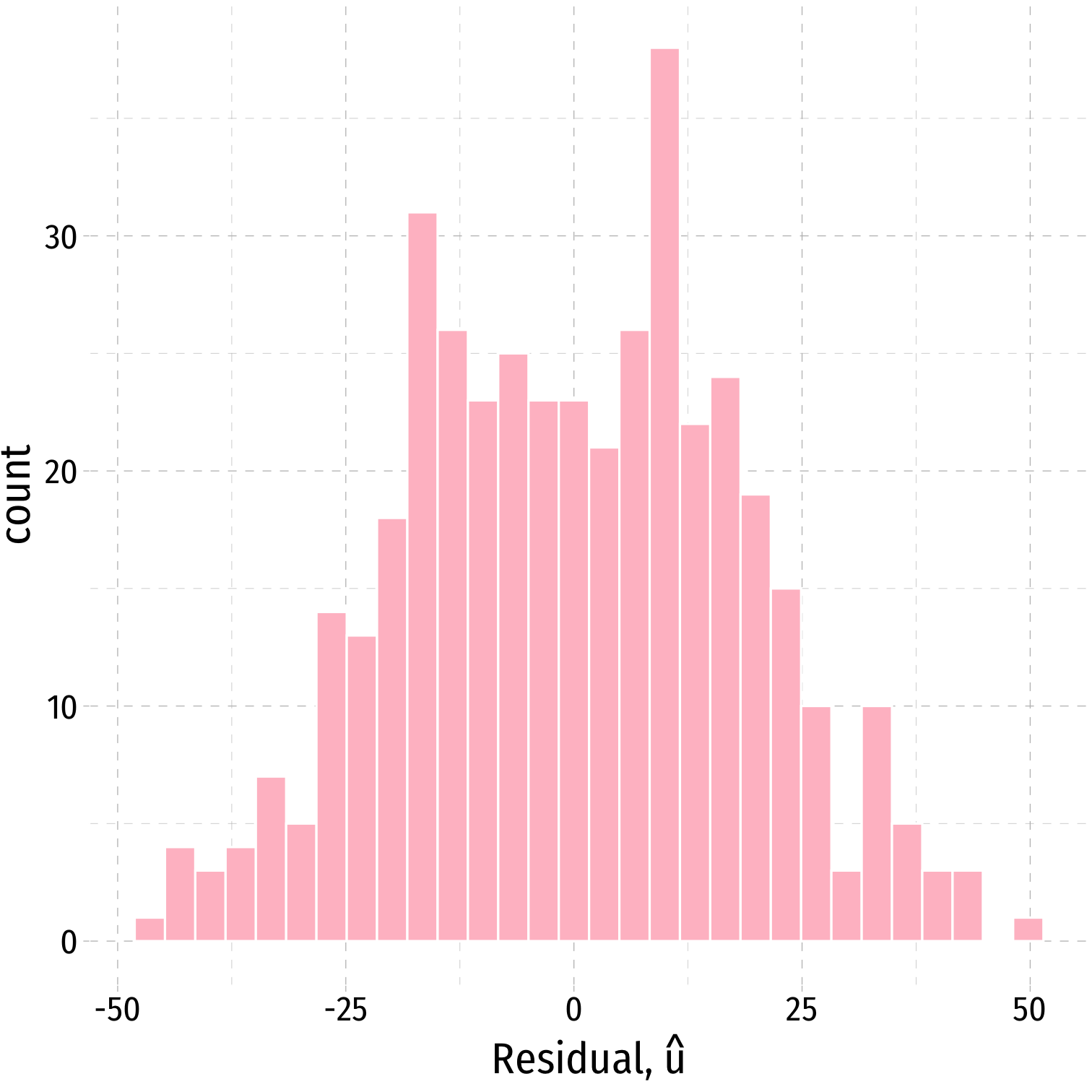
Assumptions 1 and 2 assume that errors are coming from the same (normal) distribution u∼N(0,σu)
- Assumption 1: E[u]=0
- Assumption 2: sd(u|X)=σu
- virtually always unknown...
We often can visually check by plotting a histogram of u
Plotting Residuals
ggplot(data = aug_reg)+ aes(x = .resid)+ geom_histogram(color="white", fill = "pink")+ labs(x = expression(paste("Residual, ", hat(u))))+ theme_pander(base_family = "Fira Sans Condensed", base_size=20)Plotting Residuals
ggplot(data = aug_reg)+ aes(x = .resid)+ geom_histogram(color="white", fill = "pink")+ labs(x = expression(paste("Residual, ", hat(u))))+ theme_pander(base_family = "Fira Sans Condensed", base_size=20)
Plotting Residuals
ggplot(data = aug_reg)+ aes(x = .resid)+ geom_histogram(color="white", fill = "pink")+ labs(x = expression(paste("Residual, ", hat(u))))+ theme_pander(base_family = "Fira Sans Condensed", base_size=20)- Just to check:
aug_reg %>% summarize(E_u = mean(.resid), sd_u = sd(.resid))| E_u | sd_u |
|---|---|
| 3.7e-13 | 18.6 |
Residual Plot
- We often plot a residual plot to see any odd patterns about residuals
- x-axis are X values (
str) - y-axis are u values (
.resid)
- x-axis are X values (
ggplot(data = aug_reg)+ aes(x = str, y = .resid)+ geom_point(color="blue")+ geom_hline(aes(yintercept = 0), color="red")+ labs(x = "Student to Teacher Ratio", y = expression(paste("Residual, ", hat(u))))+ theme_pander(base_family = "Fira Sans Condensed", base_size=20)Residual Plot
- We often plot a residual plot to see any odd patterns about residuals
- x-axis are X values (
str) - y-axis are u values (
.resid)
- x-axis are X values (
ggplot(data = aug_reg)+ aes(x = str, y = .resid)+ geom_point(color="blue")+ geom_hline(aes(yintercept = 0), color="red")+ labs(x = "Student to Teacher Ratio", y = expression(paste("Residual, ", hat(u))))+ theme_pander(base_family = "Fira Sans Condensed", base_size=20)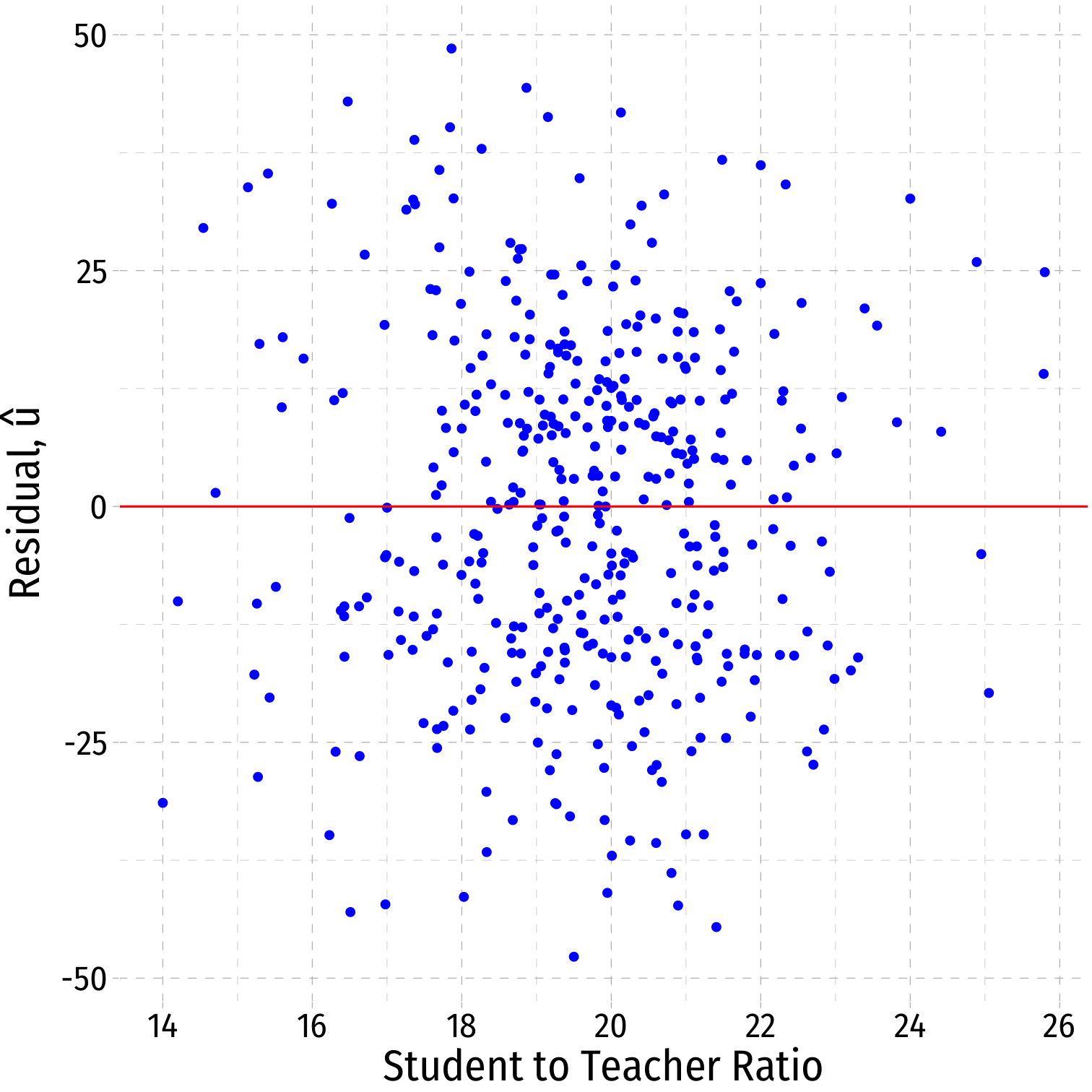
Problem: Heteroskedasticity
Homoskedasticity
"Homoskedasticity:" variance of the residuals over X is constant, written: var(u|X)=σ2u
Knowing the value of X does not affect the variance (spread) of the errors

Heteroskedasticity I
"Heteroskedasticity:" variance of the residuals over X is NOT constant: var(u|X)≠σ2u
This does not cause ^β1 to be biased, but it does cause the standard error of ^β1 to be incorrect
This does cause a problem for inference!

Heteroskedasticity II
- Recall the formula for the standard error of ^β1:
se(^β1)=√var(^β1)=SER√n×sd(X)
- This actually assumes homoskedasticity
Heteroskedasticity III
- Under heteroskedasticity, the standard error of ^β1 mutates to:
se(^β1)=√n∑i=1(Xi−ˉX)2ˆu2[n∑i=1(Xi−ˉX)2]2
This is a heteroskedasticity-robust (or just "robust") method of calculating se(^β1)
Don't learn formula, do learn what heteroskedasticity is and how it affects our model!
Visualizing Heteroskedasticity I
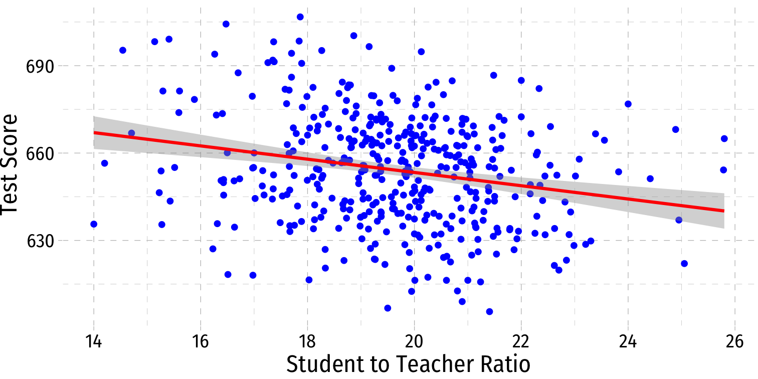
- Our original scatterplot with regression line
Visualizing Heteroskedasticity I
Our original scatterplot with regression line
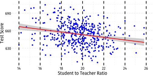
Does the spread of the errors change over different values of str?
- No: homoskedastic
- Yes: heteroskedastic

Visualizing Heteroskedasticity I
Our original scatterplot with regression line
Does the spread of the errors change over different values of str?
- No: homoskedastic
- Yes: heteroskedastic
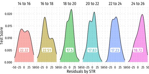
Heteroskedasticity: Another View
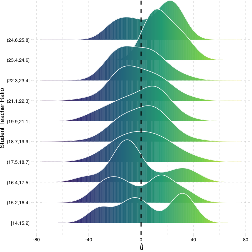
Using the
ggridgespackagePlotting the (conditional) distribution of errors by STR
See that the variation in errors (ˆu) changes across class sizes!
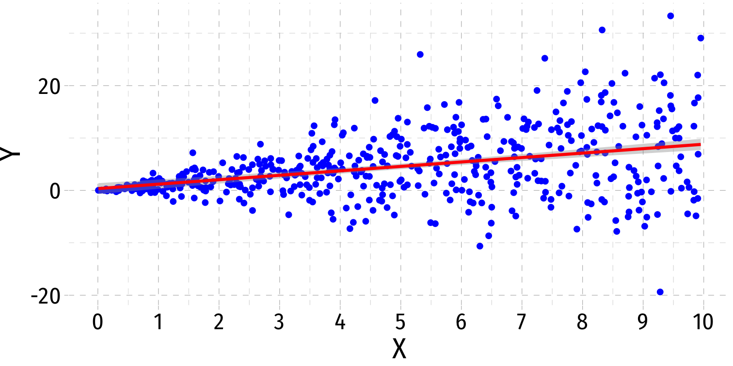
More Obvious Heteroskedasticity
- Visual cue: data is "fan-shaped"
- Data points are closer to line in some areas
- Data points are more spread from line in other areas
More Obvious Heteroskedasticity
- Visual cue: data is "fan-shaped"
- Data points are closer to line in some areas
- Data points are more spread from line in other areas

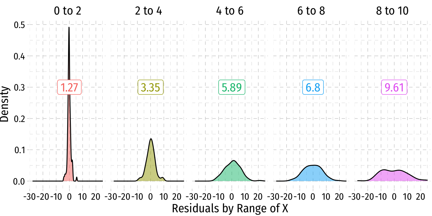
Heteroskedasticity: Another View
Using the
ggridgespackagePlotting the (conditional) distribution of errors by x
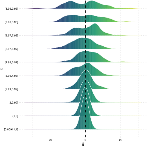
What Might Cause Heteroskedastic Errors?
^wagei=^β0+^β1educi
| Wage | |
|---|---|
| Intercept | -0.90 |
| (0.68) | |
| Years of Schooling | 0.54 *** |
| (0.05) | |
| N | 526 |
| R-Squared | 0.16 |
| SER | 3.38 |
| *** p < 0.001; ** p < 0.01; * p < 0.05. | |
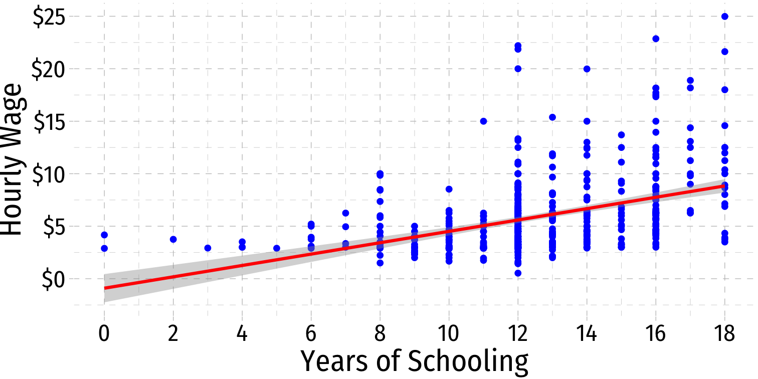
What Might Cause Heteroskedastic Errors?
^wagei=^β0+^β1educi
| Wage | |
|---|---|
| Intercept | -0.90 |
| (0.68) | |
| Years of Schooling | 0.54 *** |
| (0.05) | |
| N | 526 |
| R-Squared | 0.16 |
| SER | 3.38 |
| *** p < 0.001; ** p < 0.01; * p < 0.05. | |
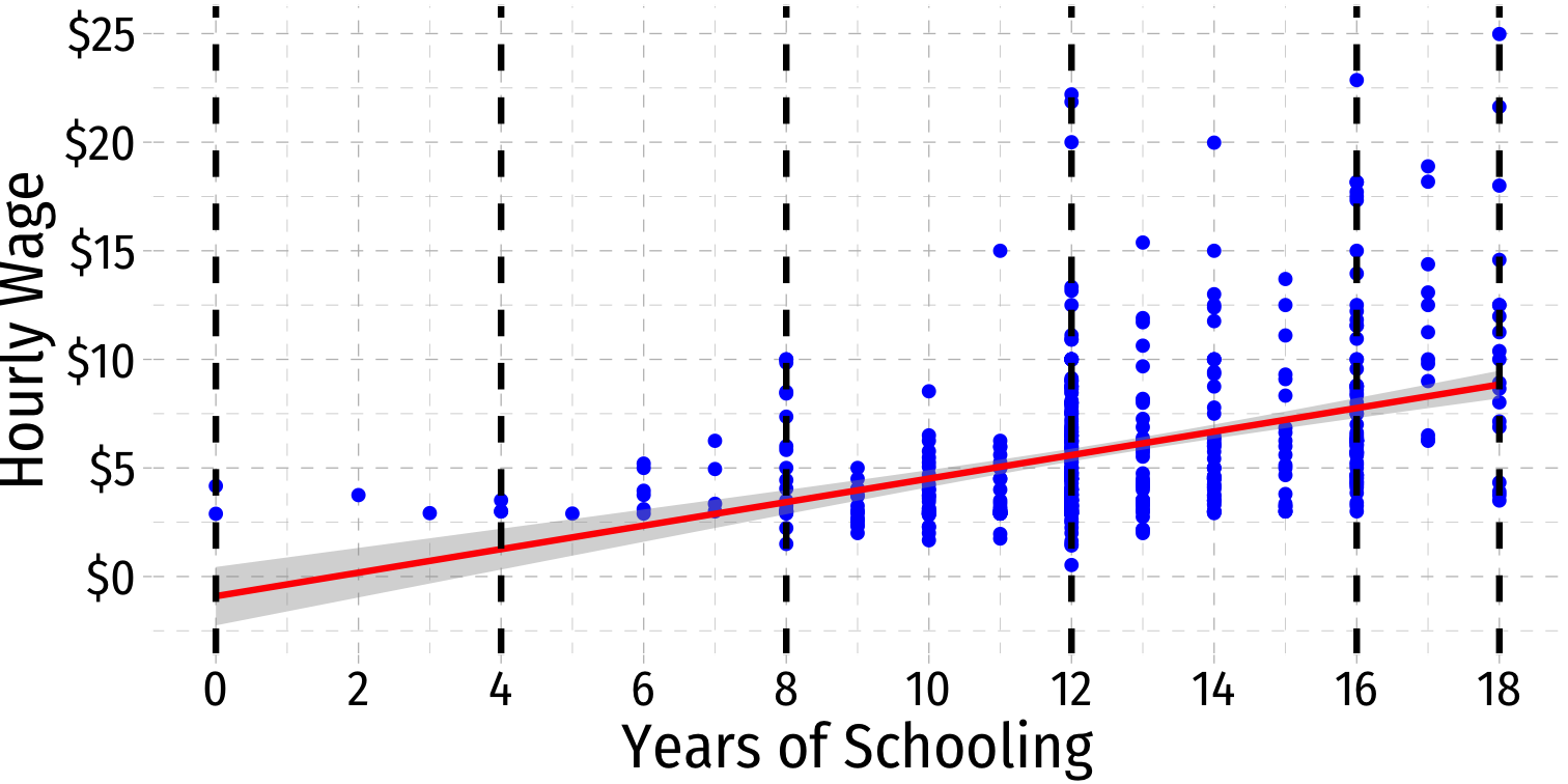
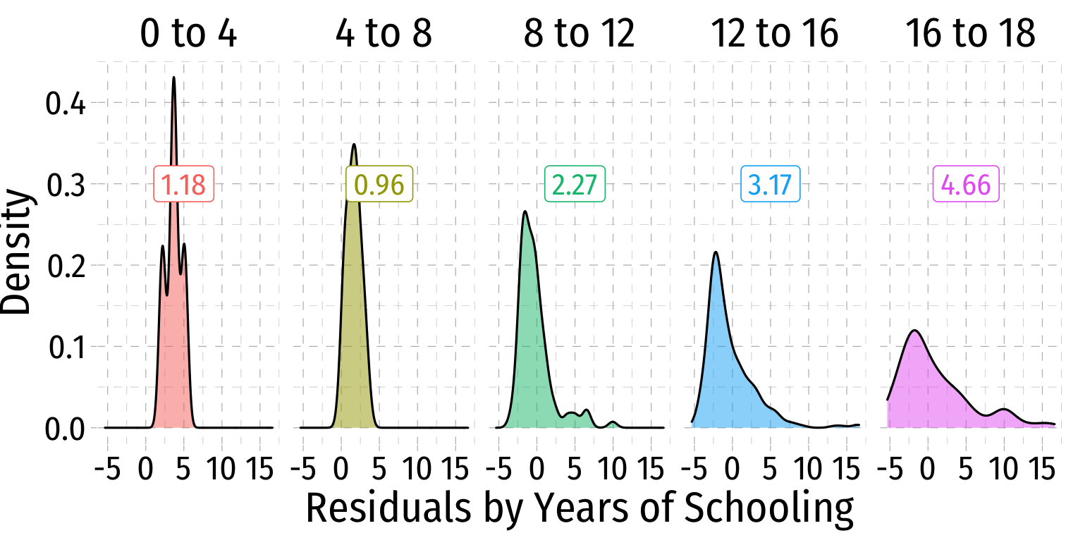
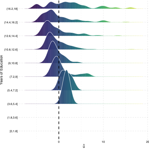
Heteroskedasticity: Another View
Using the
ggridgespackagePlotting the (conditional) distribution of errors by education
Detecting Heteroskedasticity I
- Several tests to check if data is heteroskedastic
- One common test is Breusch-Pagan test
- Can use
bptest()withlmtestpackage inR- H0: homoskedastic
- If p-value < 0.05, reject H0⟹ heteroskedastic
Detecting Heteroskedasticity I
- Several tests to check if data is heteroskedastic
- One common test is Breusch-Pagan test
- Can use
bptest()withlmtestpackage inR- H0: homoskedastic
- If p-value < 0.05, reject H0⟹ heteroskedastic
# install.packages("lmtest")library("lmtest")bptest(school_reg)## ## studentized Breusch-Pagan test## ## data: school_reg## BP = 5.7936, df = 1, p-value = 0.01608Detecting Heteroskedasticity II
- How about our wage regression?
# install.packages("lmtest")library("lmtest")bptest(wage_reg)## ## studentized Breusch-Pagan test## ## data: wage_reg## BP = 15.306, df = 1, p-value = 9.144e-05Fixing Heteroskedasticity I
Heteroskedasticity is easy to fix with software that can calculate robust standard errors (using the more complicated formula above)
Easiest method is to use
estimatrpackagelm_robust()command (instead oflm) to run regression- set
se_type="stata"to calculate robust SEs using the formula above
#install.packages("estimatr")library(estimatr)school_reg_robust <-lm_robust(testscr ~ str, data = CASchool, se_type = "stata")school_reg_robust## Estimate Std. Error t value Pr(>|t|) CI Lower CI Upper## (Intercept) 698.932952 10.3643599 67.436191 9.486678e-227 678.560192 719.305713## str -2.279808 0.5194892 -4.388557 1.446737e-05 -3.300945 -1.258671## DF## (Intercept) 418## str 418Fixing Heteroskedasticity II
library(huxtable)huxreg("Normal" = school_reg, "Robust" = school_reg_robust, coefs = c("Intercept" = "(Intercept)", "STR" = "str"), statistics = c("N" = "nobs", "R-Squared" = "r.squared", "SER" = "sigma"), number_format = 2)| Normal | Robust | |
|---|---|---|
| Intercept | 698.93 *** | 698.93 *** |
| (9.47) | (10.36) | |
| STR | -2.28 *** | -2.28 *** |
| (0.48) | (0.52) | |
| N | 420 | 420 |
| R-Squared | 0.05 | 0.05 |
| SER | 18.58 | |
| *** p < 0.001; ** p < 0.01; * p < 0.05. | ||
Assumption 3: No Serial Correlation
Errors are not correlated across observations: cor(ui,uj)=0∀i≠j
For simple cross-sectional data, this is rarely an issue
Time-series & panel data nearly always contain serial correlation or autocorrelation between errors
Errors may be clustered
- by group: e.g. all observations from Maryland, all observations from Virginia, etc.
- by time: GDP in 2006 around the world, GDP in 2008 around the world, etc.
We'll deal with these fixes when we talk about panel data (or time-series if necessary)

Outliers
Outliers Can Bias OLS! I
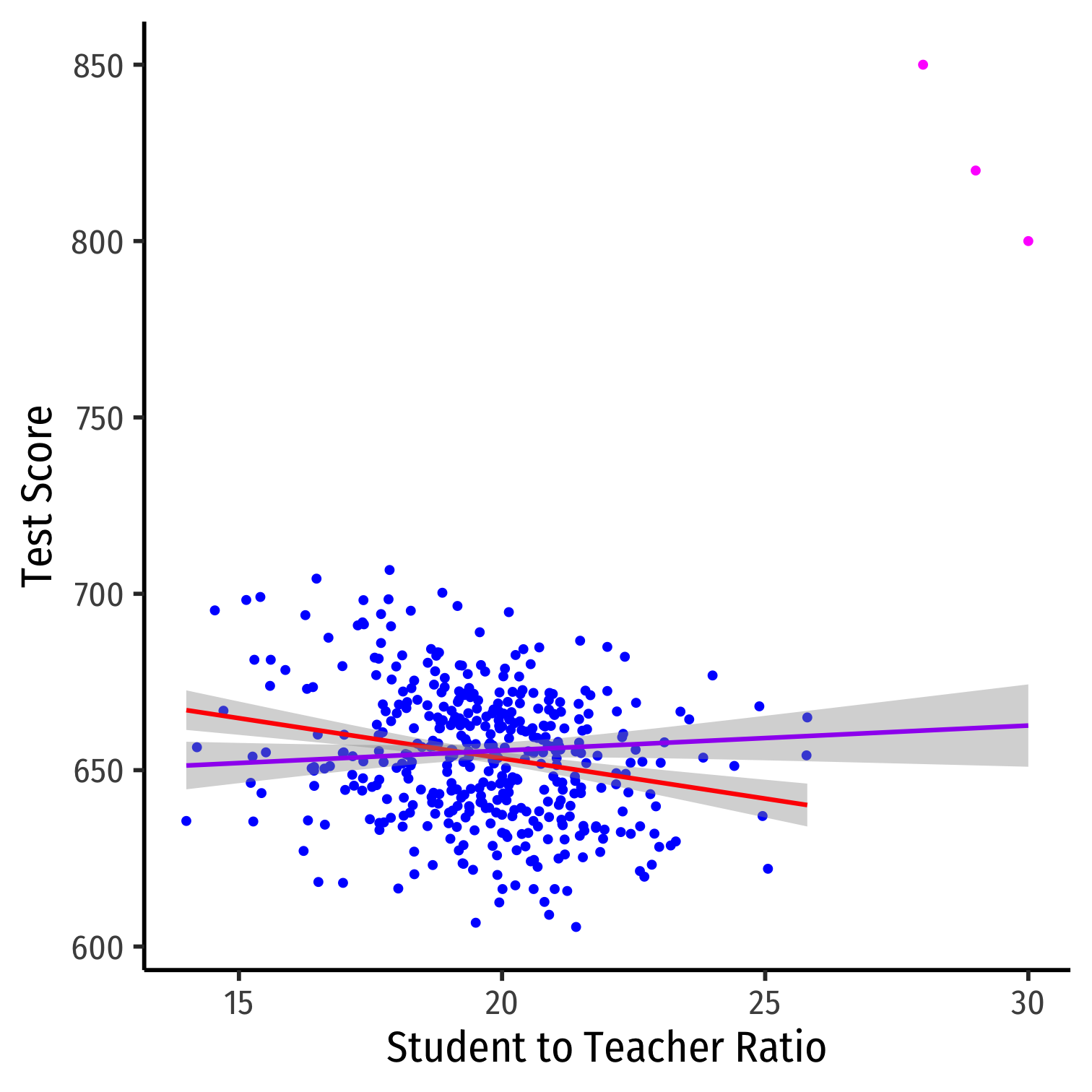
Outliers can affect the slope (and intercept) of the line and add bias
- May be result of human error (measurement, transcribing, etc)
- May be meaningful and accurate
In any case, compare how including/dropping outliers affects regression and always discuss outliers!
Outliers Can Bias OLS! II
huxreg("No Outliers" = school_reg, "Outliers" = school_outlier_reg, coefs = c("Intercept" = "(Intercept)", "STR" = "str"), statistics = c("N" = "nobs", "R-Squared" = "r.squared", "SER" = "sigma"), number_format = 2)| No Outliers | Outliers | |
|---|---|---|
| Intercept | 698.93 *** | 641.40 *** |
| (9.47) | (11.21) | |
| STR | -2.28 *** | 0.71 |
| (0.48) | (0.57) | |
| N | 420 | 423 |
| R-Squared | 0.05 | 0.00 |
| SER | 18.58 | 23.76 |
| *** p < 0.001; ** p < 0.01; * p < 0.05. | ||

Detecting Outliers
- The
carpackage has anoutlierTestcommand to run on the regression
library("car")# Use Bonferonni test outlierTest(school_outlier_reg) # will point out which obs #s seem outliers## rstudent unadjusted p-value Bonferroni p## 422 8.822768 3.0261e-17 1.2800e-14## 423 7.233470 2.2493e-12 9.5147e-10## 421 6.232045 1.1209e-09 4.7414e-07# find these observationsCA.outlier %>% slice(c(422,423,421))| observat | district | testscr | str |
|---|---|---|---|
| 422 | Crazy School 2 | 850 | 28 |
| 423 | Crazy School 3 | 820 | 29 |
| 421 | Crazy School 1 | 800 | 30 |