Recall: The Two Big Problems with Data
- We use econometrics to identify causal relationships and make inferences about them
Problem for identification: endogeneity
- X is exogenous if cor(x,u)=0
- X is endogenous if cor(x,u)≠0
Problem for inference: randomness
- Data is random due to natural sampling variation
- Taking one sample of a population will yield slightly different information than another sample of the same population


Why Sample vs. Population Matters

Population
Why Sample vs. Population Matters
Population
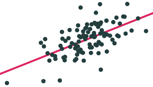
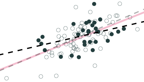
Population relationship
Yi=3.24+0.44Xi+ui
Yi=β0+β1Xi+ui
Why Sample vs. Population Matters
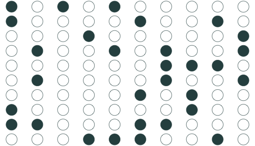
Sample 1: 30 random individuals
Why Sample vs. Population Matters
Sample 1: 30 random individuals
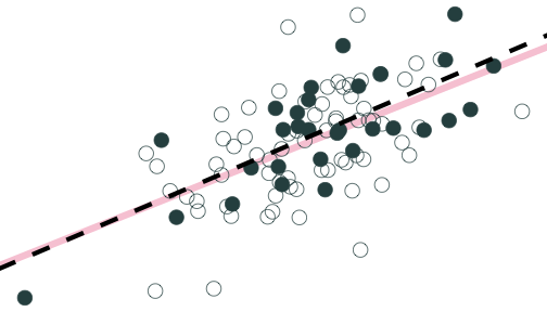
Population relationship
Yi=3.24+0.44Xi+ui
Sample relationship
ˆYi=3.19+0.47Xi
Why Sample vs. Population Matters
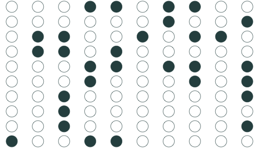
Sample 2: 30 random individuals
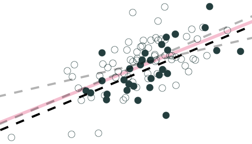
Population relationship
Yi=3.24+0.44Xi+ui
Sample relationship
ˆYi=4.26+0.25Xi
Why Sample vs. Population Matters
Sample 3: 30 random individuals
Population relationship
Yi=3.24+0.44Xi+ui
Sample relationship
ˆYi=2.91+0.46Xi
Why Sample vs. Population Matters
Let's repeat this process 10,000 times!
This exercise is called a (Monte Carlo) simulation
- I'll show you how to do this next class with the
inferpackage
- I'll show you how to do this next class with the

Why Sample vs. Population Matters
On average estimated regression lines from our hypothetical samples provide an unbiased estimate of the true population regression line E[^β1]=β1
However, any individual line (any one sample) can miss the mark
This leads to uncertainty about our estimated regression line
- Remember, we only have one sample in reality!
- This is why we care about the standard error of our line: se(^β1)!

Estimation and Statistical Inference
Our problem with uncertainty is we don’t know whether our sample estimate is close or far from the unknown population parameter
But we can use our errors to learn how well our model statistics likely estimate the true parameters
Use ^β1 and its standard error, se(^β1) for statistical inference about true β1
We have two options...
Estimation and Statistical Inference

Point estimate
Use our ^β1 & se(^β1) to determine if statistically significant evidence to reject a hypothesized β1
Reporting a single value (^β1) is often not going to be the true population parameter (β1)

Confidence interval
- Use our ^β1 & se(^β1) to create a range of values that gives us a good chance of capturing the true β1
Accuracy vs. Precision

- More typical in econometrics to do hypothesis testing (next class)
Generating Confidence Intervals
We can generate our confidence interval by generating a “bootstrap” sampling distribution
This takes our sample data, and resamples it by selecting random observations with replacement
This allows us to approximate the sampling distribution of ^β1 by simulation!

Confidence Intervals Using the infer Package

- The
inferpackage allows you to do statistical inference in atidyway, following the philosophy of thetidyverse
# install first!install.packages("infer")# loadlibrary(infer)Confidence Intervals with the infer Package I
inferallows you to run through these steps manually to understand the process:
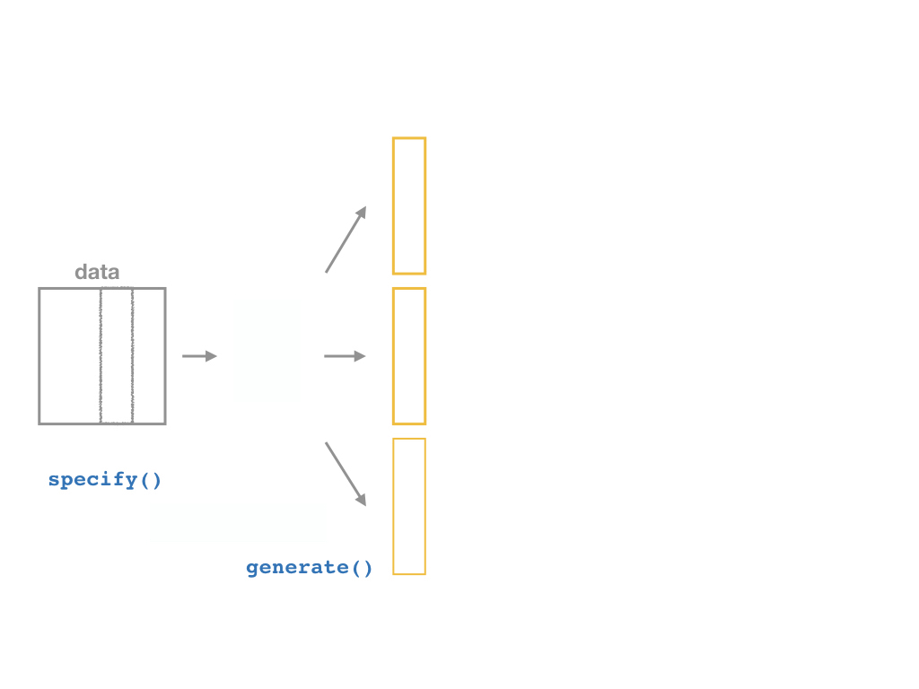
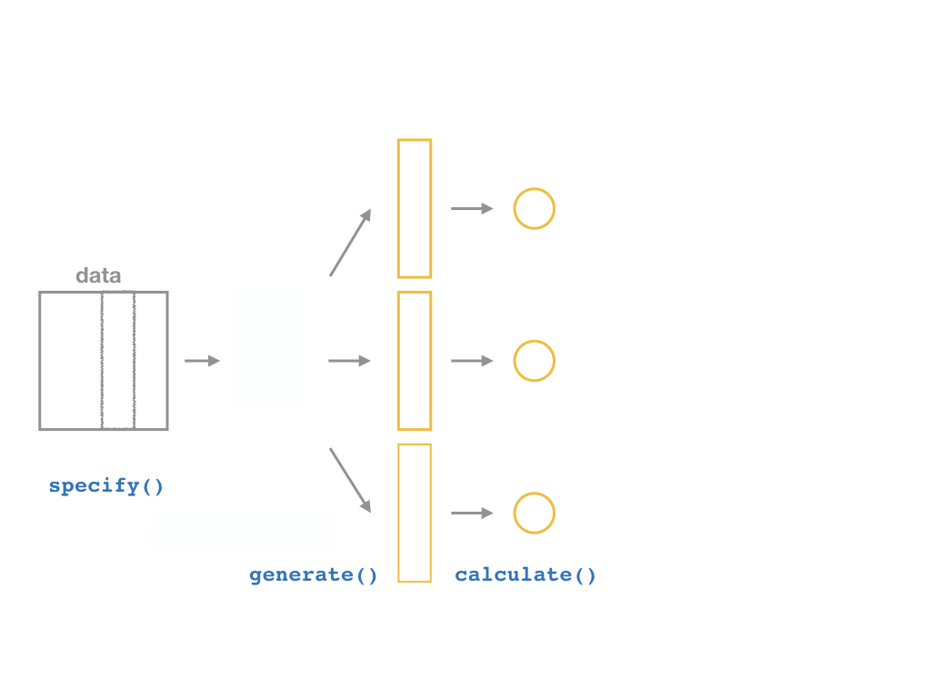
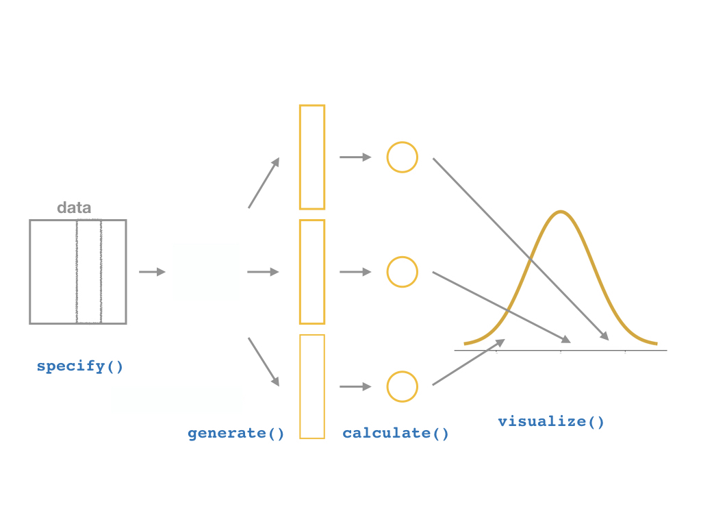
specify()a modelgenerate()a bootstrap distributioncalculate()the confidence intervalvisualize()with a histogram (optional)
Confidence Intervals with the infer Package II

Confidence Intervals with the infer Package II

Confidence Intervals with the infer Package II
Confidence Intervals with the infer Package II
Confidence Intervals with the infer Package II
The infer Pipeline: Specify
The infer Pipeline: Generate
Confidence Interval
- A 95% confidence interval is the middle 95% of the sampling distribution
lower <dbl> | upper <dbl> | |
|---|---|---|
| -3.340545 | -1.238815 |
sampling_dist<-ggplot(data = boot)+ aes(x = stat)+ geom_histogram(color="white", fill = "#e64173")+ labs(x = expression(hat(beta[1])))+ theme_pander(base_family = "Fira Sans Condensed", base_size=20)sampling_dist
Confidence Interval
- A confidence interval is the middle 95% of the sampling distribution
ci<-boot %>% summarize(lower = quantile(stat, 0.025), upper = quantile(stat, 0.975))cilower <dbl> | upper <dbl> | |
|---|---|---|
| -3.340545 | -1.238815 |
sampling_dist+ geom_vline(data = ci, aes(xintercept = lower), size = 1, linetype="dashed")+ geom_vline(data = ci, aes(xintercept = upper), size = 1, linetype="dashed")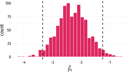
The infer Pipeline: Confidence Interval
Specify
Generate
Calculate
Visualize
%>% visualize()
CASchool %>% #<< # save this specify(testscr ~ str) %>% generate(reps = 1000, type = "bootstrap") %>% calculate(stat = "slope") %>% visualize()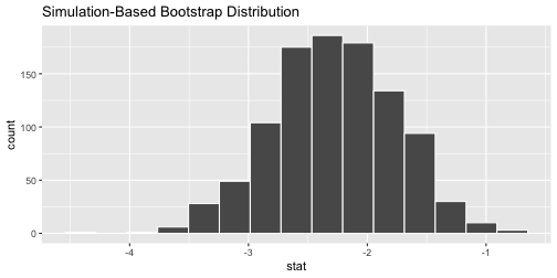
visualize()is just a wrapper forggplot()
The infer Pipeline: Confidence Interval
Specify
Generate
Calculate
Visualize
%>% visualize()
CASchool %>% #<< # save this specify(testscr ~ str) %>% generate(reps = 1000, type = "bootstrap") %>% calculate(stat = "slope") %>% visualize()+shade_ci(endpoints = our_CI)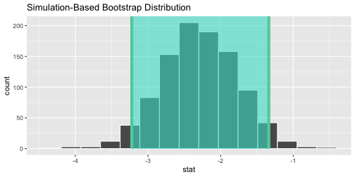
- If we have our confidence levels saved (
our_CI) we canshade_ci()ininfer'svisualize()function
Confidence Intervals
- In general, a confidence interval (CI) takes a point estimate and extrapolates it within some margin of error (MOE):
([ estimate - MOE ], [ estimate + MOE ])
- The main question is, how confident do we want to be that our interval contains the true parameter?
- Larger confidence level, larger margin of error (and thus larger interval)
Confidence Intervals
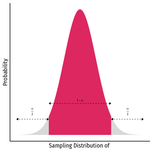
(1−α) is the confidence level of our confidence interval
- α is the “significance level” that we use in hypothesis testing
- α= probability that the true parameter is not contained within our interval
Typical levels: 90%, 95%, 99%
- 95% is especially common, α=0.05
Confidence Levels
Depending on our confidence level, we are essentially looking for the middle (1−α)% of the sampling distribution
This puts α in the tails; α2 in each tail
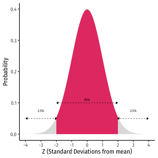
Confidence Levels and the Empirical Rule
Recall the 68-95-99.7% empirical rule for (standard) normal distributions!†
95% of data falls within 2 standard deviations of the mean
Thus, in 95% of samples, the true parameter is likely to fall within about 2 standard deviations of the sample estimate
† I’m playing fast and loose here, we can’t actually use the normal distribution, we use the Student’s t-distribution with n-k-1 degrees of freedom. But there’s no need to complicate things you don’t need to know about. Look at today’s class notes for more.