3.8 — Polynomial Regression
ECON 480 • Econometrics • Fall 2021
Ryan Safner
Assistant Professor of Economics
safner@hood.edu
ryansafner/metricsF21
metricsF21.classes.ryansafner.com
Linear Regression
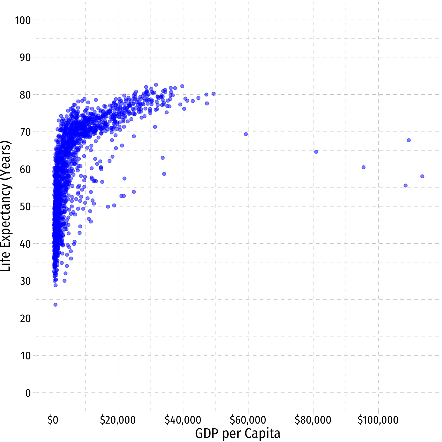
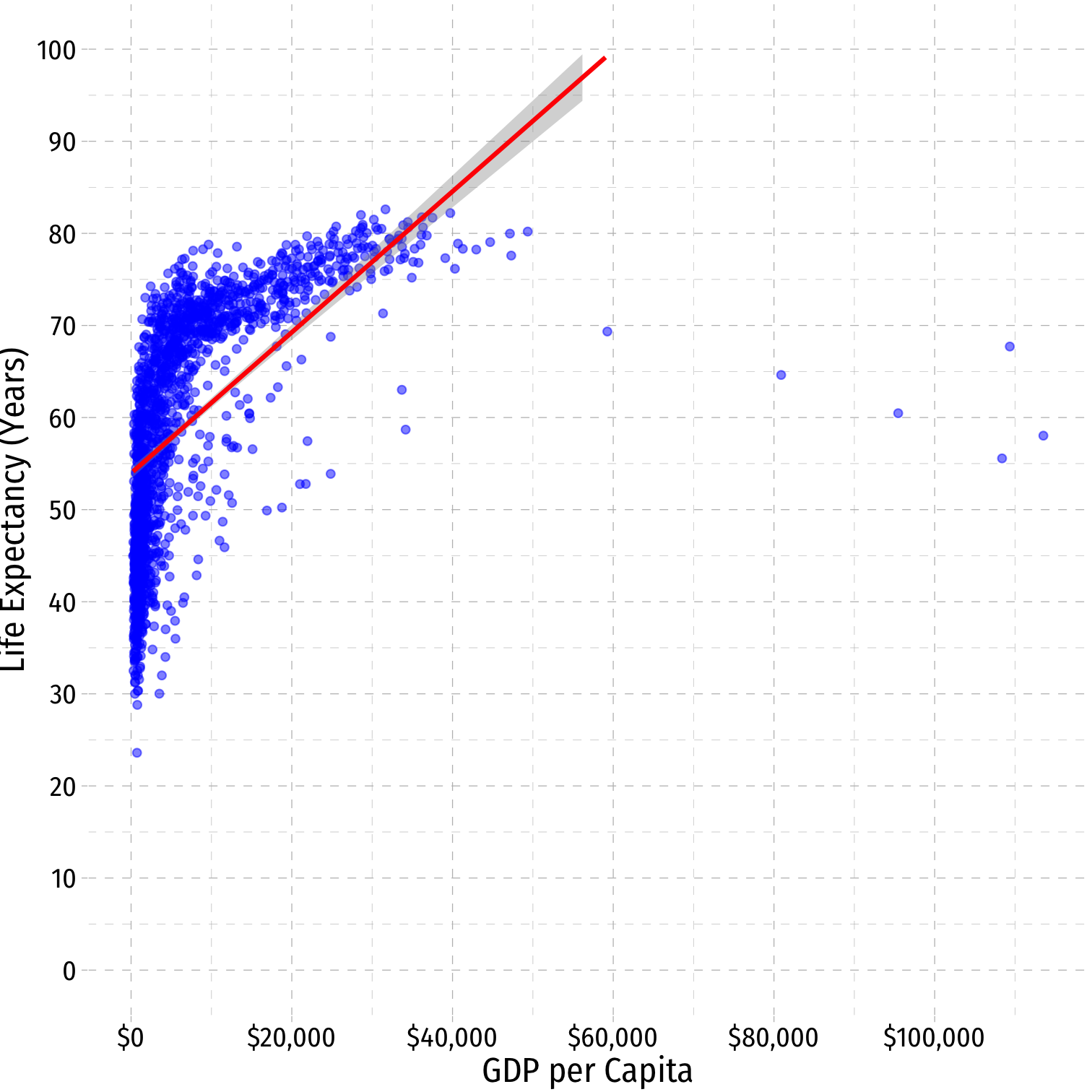
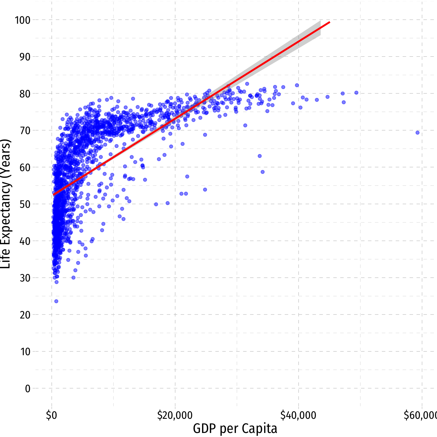
OLS is commonly known as “linear_ regression” as it fits a straight line to data points
Often, data and relationships between variables may not be linear
Linear Regression
OLS is commonly known as “linear_ regression” as it fits a straight line to data points
Often, data and relationships between variables may not be linear
Linear Regression
OLS is commonly known as “linear_ regression” as it fits a straight line to data points
Often, data and relationships between variables may not be linear
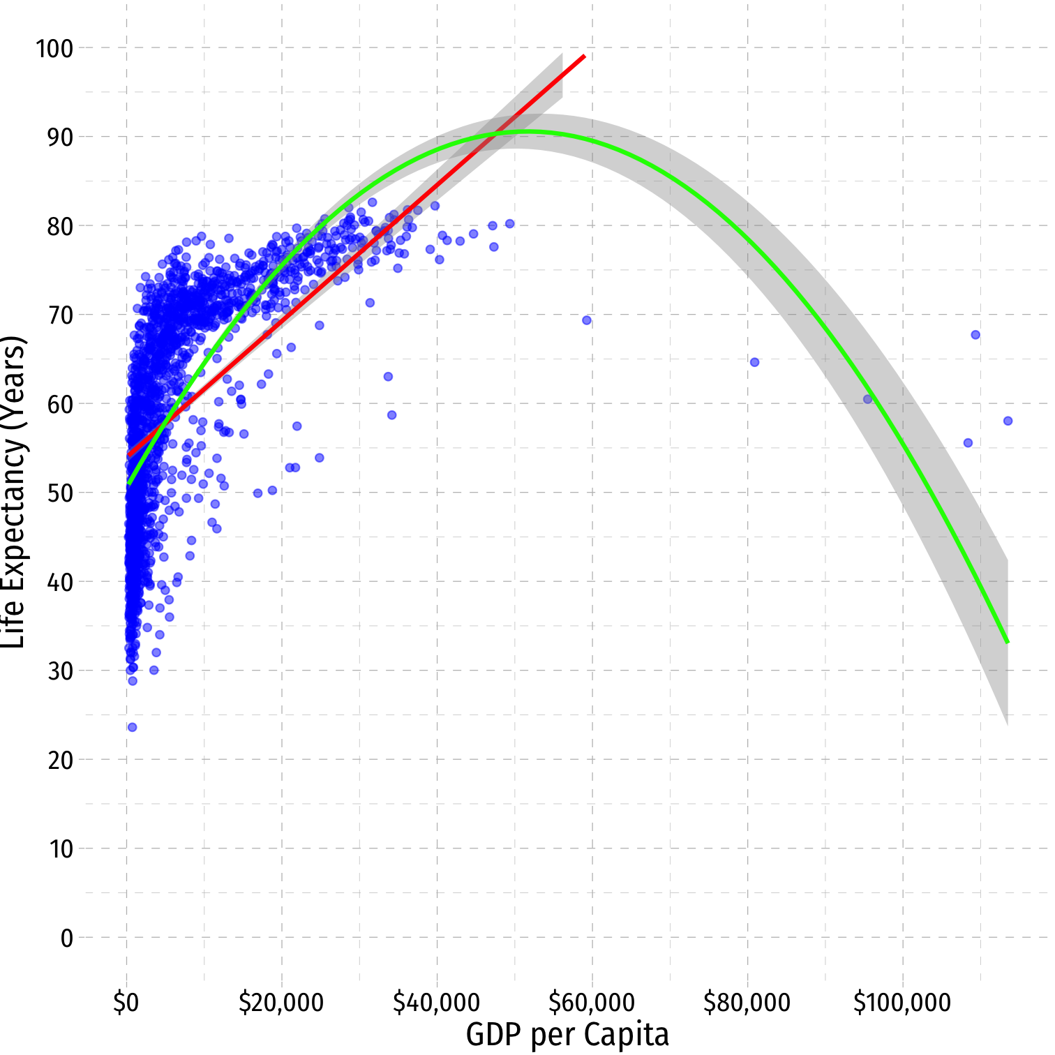
^Life Expectancyi=^β0+^β1GDPi
Linear Regression
OLS is commonly known as “linear_ regression” as it fits a straight line to data points
Often, data and relationships between variables may not be linear
^Life Expectancyi=^β0+^β1GDPi
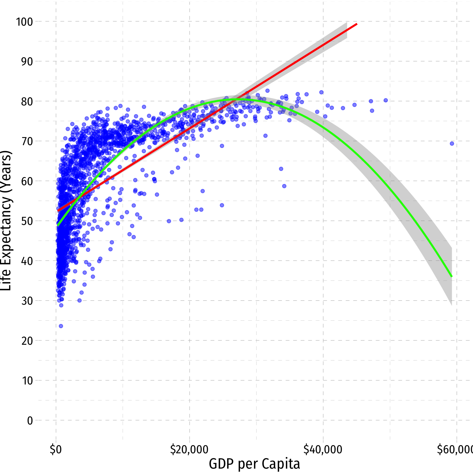
^Life Expectancyi=^β0+^β1GDPi+^β2GDP2i
Linear Regression
OLS is commonly known as “linear_ regression” as it fits a straight line to data points
Often, data and relationships between variables may not be linear
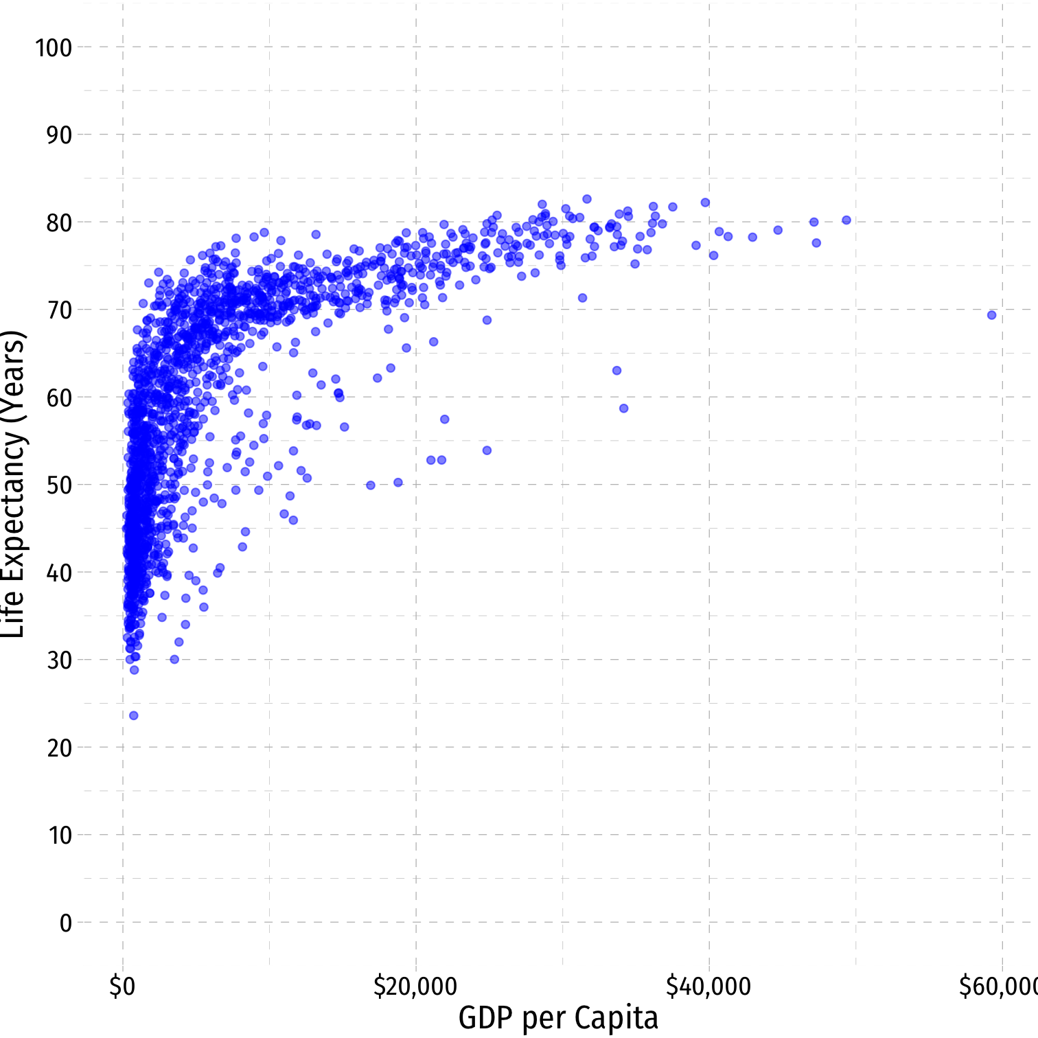
Get rid of the outliers (>$60,000)
Linear Regression
OLS is commonly known as “linear_ regression” as it fits a straight line to data points
Often, data and relationships between variables may not be linear
Get rid of the outliers (>$60,000)
^Life Expectancyi=^β0+^β1GDPi
Linear Regression
OLS is commonly known as “linear_ regression” as it fits a straight line to data points
Often, data and relationships between variables may not be linear
Get rid of the outliers (>$60,000)
^Life Expectancyi=^β0+^β1GDPi
^Life Expectancyi=^β0+^β1GDPi+^β2GDP2i
Linear Regression
OLS is commonly known as “linear_ regression” as it fits a straight line to data points
Often, data and relationships between variables may not be linear
Get rid of the outliers (>$60,000)
^Life Expectancyi=^β0+^β1GDPi
^Life Expectancyi=^β0+^β1GDPi+^β2GDP2i
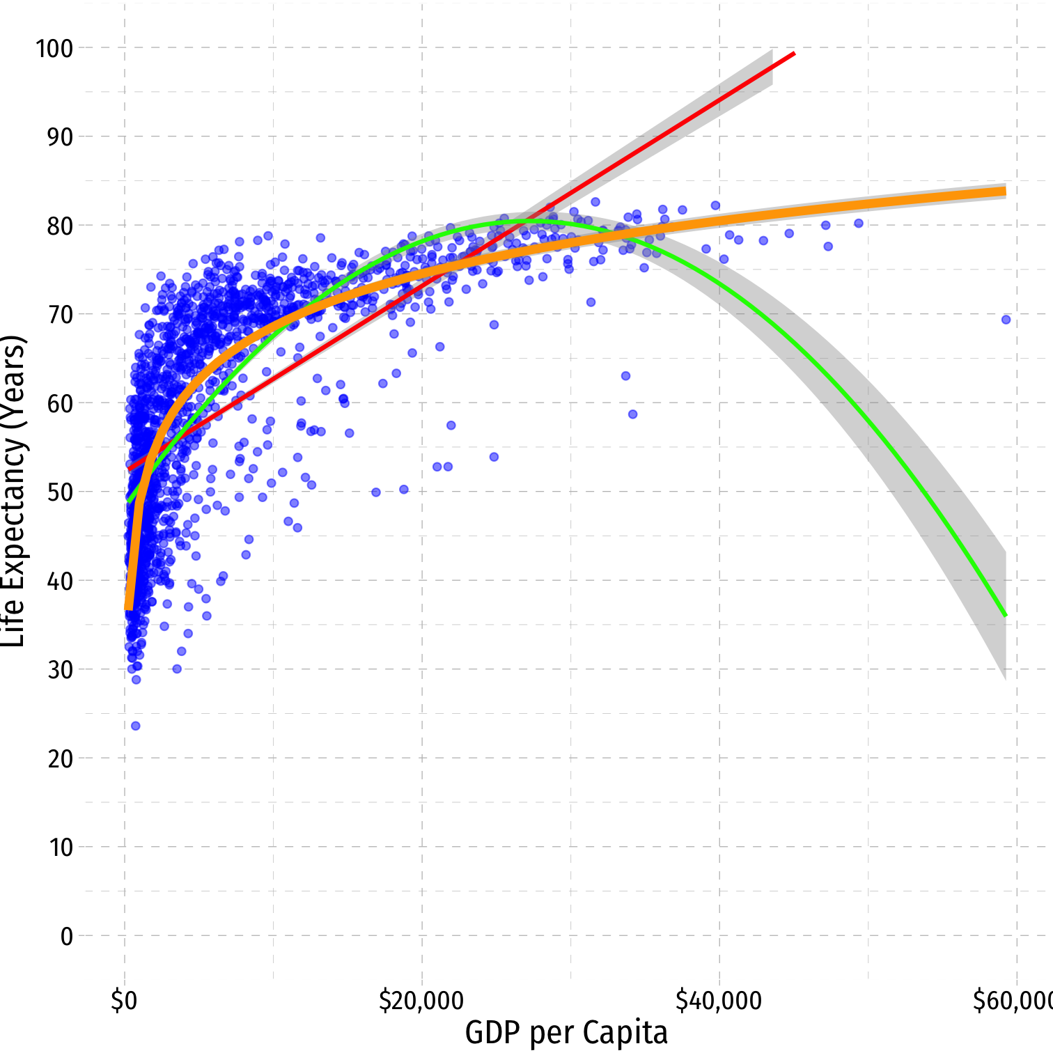
^Life Expectancyi=^β0+^β1ln(GDPi)
Nonlinear Effects in Linear Regression
Despite being “linear regression”, OLS can handle this with an easy fix
OLS requires all parameters (i.e. the β's) to be linear, the regressors (X's) can be nonlinear:
Nonlinear Effects in Linear Regression
Despite being “linear regression”, OLS can handle this with an easy fix
OLS requires all parameters (i.e. the β's) to be linear, the regressors (X's) can be nonlinear:
Yi=β0+β1X2i✅
Nonlinear Effects in Linear Regression
Despite being “linear regression”, OLS can handle this with an easy fix
OLS requires all parameters (i.e. the β's) to be linear, the regressors (X's) can be nonlinear:
Yi=β0+β1X2i✅
Yi=β0+β21Xi❌
Nonlinear Effects in Linear Regression
Despite being “linear regression”, OLS can handle this with an easy fix
OLS requires all parameters (i.e. the β's) to be linear, the regressors (X's) can be nonlinear:
Yi=β0+β1X2i✅
Yi=β0+β21Xi❌
Yi=β0+β1√Xi✅
Nonlinear Effects in Linear Regression
Despite being “linear regression”, OLS can handle this with an easy fix
OLS requires all parameters (i.e. the β's) to be linear, the regressors (X's) can be nonlinear:
Yi=β0+β1X2i✅
Yi=β0+β21Xi❌
Yi=β0+β1√Xi✅
Yi=β0+√β1Xi❌
Nonlinear Effects in Linear Regression
Despite being “linear regression”, OLS can handle this with an easy fix
OLS requires all parameters (i.e. the β's) to be linear, the regressors (X's) can be nonlinear:
Yi=β0+β1X2i✅
Yi=β0+β21Xi❌
Yi=β0+β1√Xi✅
Yi=β0+√β1Xi❌
Yi=β0+β1(X1i×X2i)✅
Nonlinear Effects in Linear Regression
Despite being “linear regression”, OLS can handle this with an easy fix
OLS requires all parameters (i.e. the β's) to be linear, the regressors (X's) can be nonlinear:
Yi=β0+β1X2i✅
Yi=β0+β21Xi❌
Yi=β0+β1√Xi✅
Yi=β0+√β1Xi❌
Yi=β0+β1(X1i×X2i)✅
Yi=β0+β1ln(Xi)✅
Nonlinear Effects in Linear Regression
Despite being “linear regression”, OLS can handle this with an easy fix
OLS requires all parameters (i.e. the β's) to be linear, the regressors (X's) can be nonlinear:
Yi=β0+β1X2i✅
Yi=β0+β21Xi❌
Yi=β0+β1√Xi✅
Yi=β0+√β1Xi❌
Yi=β0+β1(X1i×X2i)✅
Yi=β0+β1ln(Xi)✅
- In the end, each X is always just a number in the data, OLS can always estimate parameters for it; but plotting the modelled points (Xi,^Yi) can result in a curve!
Sources of Nonlinearities
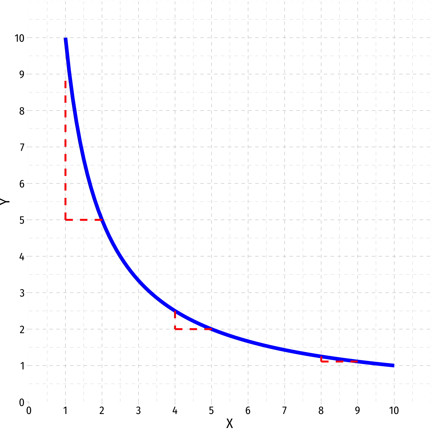
- Effect of X1→Y might be nonlinear if:
Sources of Nonlinearities
- Effect of X1→Y might be nonlinear if:
- X1→Y is different for different levels of X1
- e.g. diminishing returns: ↑X1 increases Y at a decreasing rate
- e.g. increasing returns: ↑X1 increases Y at an increasing rate
Sources of Nonlinearities
- Effect of X1→Y might be nonlinear if:
X1→Y is different for different levels of X1
- e.g. diminishing returns: ↑X1 increases Y at a decreasing rate
- e.g. increasing returns: ↑X1 increases Y at an increasing rate
X1→Y is different for different levels of X2
- e.g. interaction effects (last lesson)
Nonlinearities Alter Marginal Effects
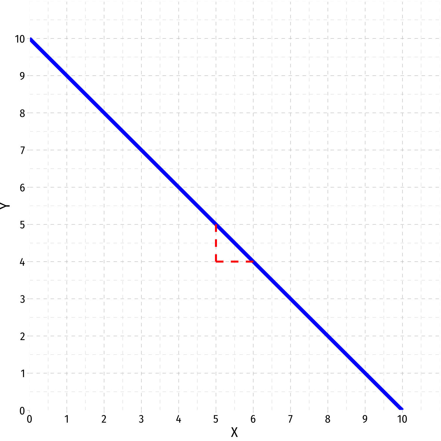
Linear: Y=^β0+^β1X
marginal effect (slope), (^β1)=ΔYΔX is constant for all X
Nonlinearities Alter Marginal Effects
Polynomial: Y=^β0+^β1X+^β2X2
Marginal effect, “slope” (≠^β1) depends on the value of X!
Sources of Nonlinearities III
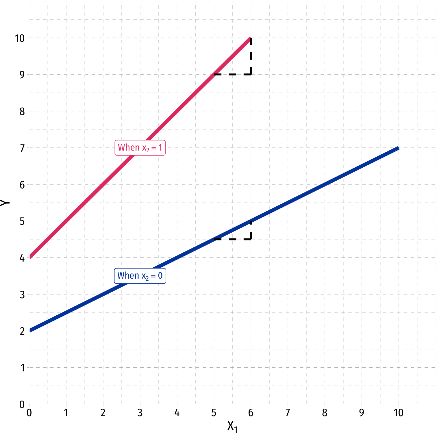
Interaction Effect: ˆY=^β0+^β1X1+^β2X2+^β3X1×X2
Marginal effect, “slope” depends on the value of X2!
Easy example: if X2 is a dummy variable:
- X2=0 (control) vs. X2=1 (treatment)
Polynomial Functions of X I
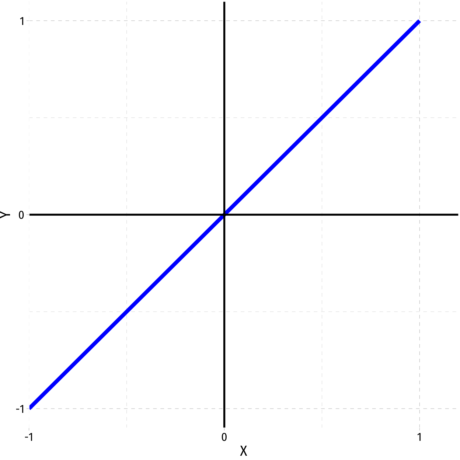
- Linear
ˆY=^β0+^β1X
Polynomial Functions of X I
- Linear
ˆY=^β0+^β1X
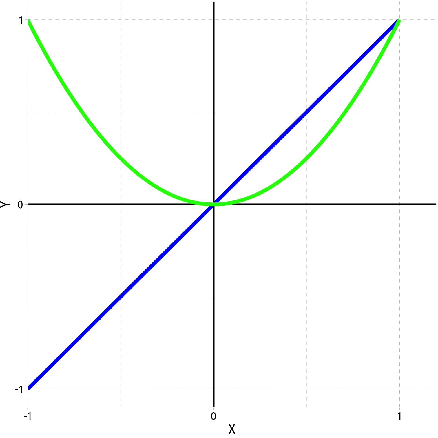
- Quadratic
ˆY=^β0+^β1X+^β2X2
Polynomial Functions of X I
- Linear
ˆY=^β0+^β1X
- Quadratic
ˆY=^β0+^β1X+^β2X2
- Cubic
ˆY=^β0+^β1X+^β2X2+^β3X3
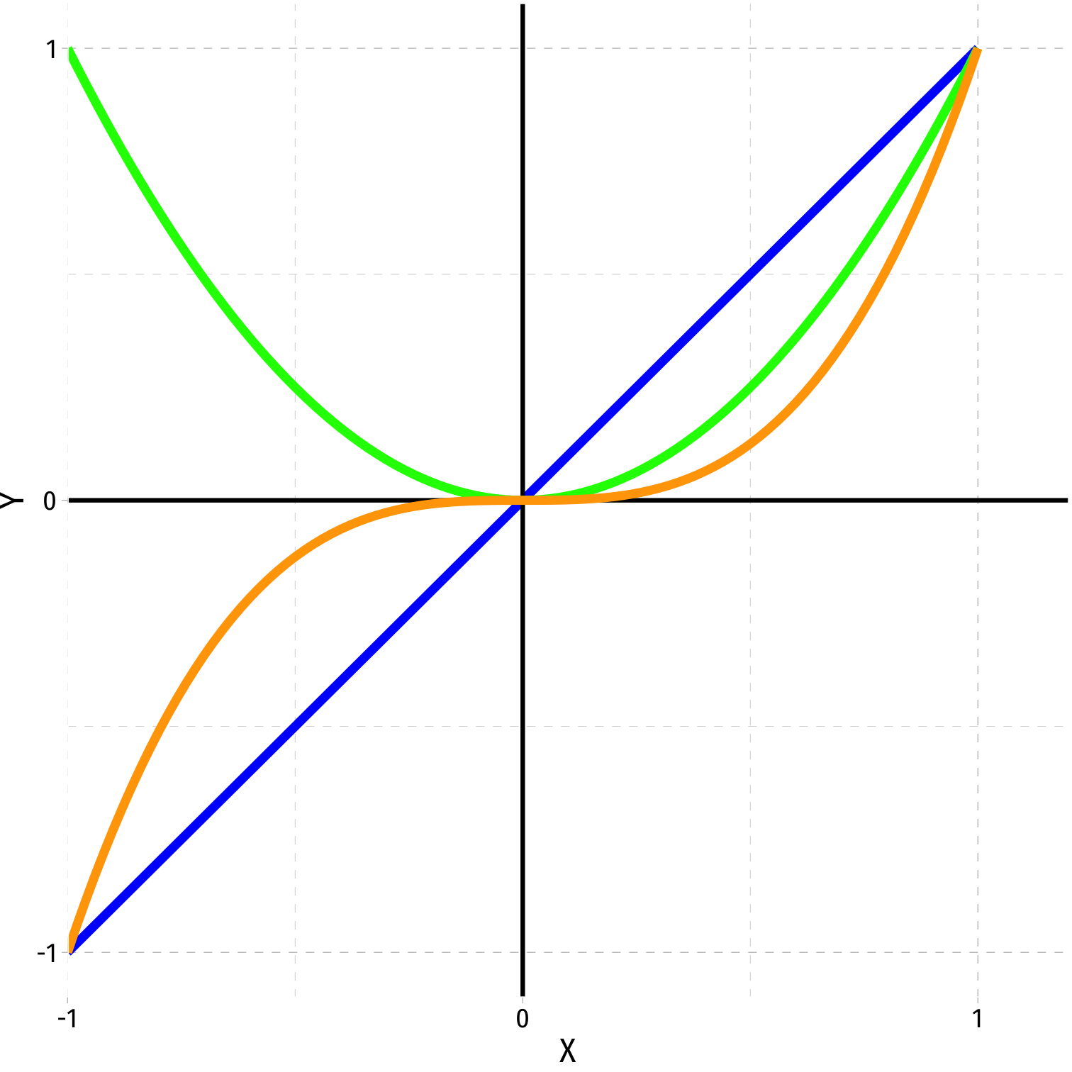
Polynomial Functions of X I
- Linear
ˆY=^β0+^β1X
- Quadratic
ˆY=^β0+^β1X+^β2X2
- Cubic
ˆY=^β0+^β1X+^β2X2+^β3X3
- Quartic
ˆY=^β0+^β1X+^β2X2+^β3X3+^β4X4
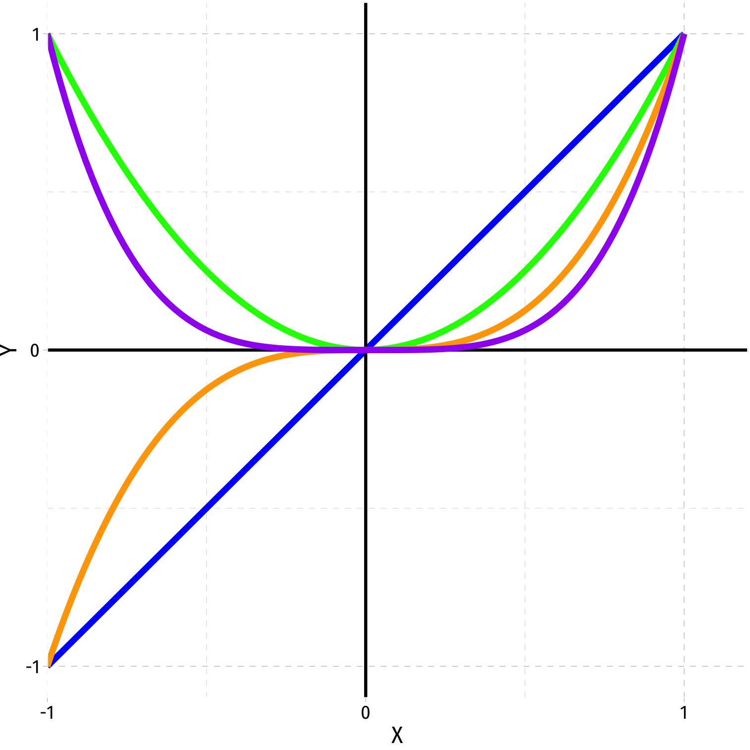
Polynomial Functions of X I
^Yi=^β0+^β1Xi+^β2X2i+⋯+^βrXri+ui
Polynomial Functions of X I
^Yi=^β0+^β1Xi+^β2X2i+⋯+^βrXri+ui
- Where r is the highest power Xi is raised to
- quadratic r=2
- cubic r=3
Polynomial Functions of X I
^Yi=^β0+^β1Xi+^β2X2i+⋯+^βrXri+ui
Where r is the highest power Xi is raised to
- quadratic r=2
- cubic r=3
The graph of an rth-degree polynomial function has (r−1) bends
Polynomial Functions of X I
^Yi=^β0+^β1Xi+^β2X2i+⋯+^βrXri+ui
Where r is the highest power Xi is raised to
- quadratic r=2
- cubic r=3
The graph of an rth-degree polynomial function has (r−1) bends
Just another multivariate OLS regression model!
The Quadratic Model
Quadratic Model
^Yi=^β0+^β1Xi+^β2X2i
- Quadratic model has X and X2 variables in it (yes, need both!)
Quadratic Model
^Yi=^β0+^β1Xi+^β2X2i
Quadratic model has X and X2 variables in it (yes, need both!)
How to interpret coefficients (betas)?
- β0 as “intercept” and β1 as “slope” makes no sense 🧐
- β1 as effect Xi→Yi holding X2i constant??†
† Note: this is not a perfect multicollinearity problem! Correlation only measures linear relationships!
- Estimate marginal effects by calculating predicted ^Yi for different levels of Xi
Quadratic Model: Calculating Marginal Effects
^Yi=^β0+^β1Xi+^β2X2i
- What is the marginal effect of ΔXi→ΔYi?
Quadratic Model: Calculating Marginal Effects
^Yi=^β0+^β1Xi+^β2X2i
What is the marginal effect of ΔXi→ΔYi?
Take the derivative of Yi with respect to Xi: ∂Yi∂Xi=^β1+2^β2Xi
Quadratic Model: Calculating Marginal Effects
^Yi=^β0+^β1Xi+^β2X2i
What is the marginal effect of ΔXi→ΔYi?
Take the derivative of Yi with respect to Xi: ∂Yi∂Xi=^β1+2^β2Xi
Marginal effect of a 1 unit change in Xi is a (^β1+2^β2Xi) unit change in Y
Quadratic Model: Example I
Example: ^Life Expectancyi=^β0+^β1GDP per capitai+^β2GDP per capita2i
- Use
gapminderpackage and data
library(gapminder)Quadratic Model: Example II
- These coefficients will be very large, so let's transform
gdpPercapto be in $1,000's
gapminder <- gapminder %>% mutate(GDP_t = gdpPercap/1000)gapminder %>% head() # look at it| ABCDEFGHIJ0123456789 |
country <fct> | continent <fct> | year <int> | lifeExp <dbl> | pop <int> | gdpPercap <dbl> | GDP_t <dbl> |
|---|---|---|---|---|---|---|
| Afghanistan | Asia | 1952 | 28.801 | 8425333 | 779.4453 | 0.7794453 |
| Afghanistan | Asia | 1957 | 30.332 | 9240934 | 820.8530 | 0.8208530 |
| Afghanistan | Asia | 1962 | 31.997 | 10267083 | 853.1007 | 0.8531007 |
| Afghanistan | Asia | 1967 | 34.020 | 11537966 | 836.1971 | 0.8361971 |
| Afghanistan | Asia | 1972 | 36.088 | 13079460 | 739.9811 | 0.7399811 |
| Afghanistan | Asia | 1977 | 38.438 | 14880372 | 786.1134 | 0.7861134 |
Quadratic Model: Example III
- Let’s also create a squared term,
gdp_sq
gapminder <- gapminder %>% mutate(GDP_sq = GDP_t^2)gapminder %>% head() # look at it| ABCDEFGHIJ0123456789 |
country <fct> | continent <fct> | year <int> | lifeExp <dbl> | pop <int> | gdpPercap <dbl> | GDP_t <dbl> | |
|---|---|---|---|---|---|---|---|
| Afghanistan | Asia | 1952 | 28.801 | 8425333 | 779.4453 | 0.7794453 | |
| Afghanistan | Asia | 1957 | 30.332 | 9240934 | 820.8530 | 0.8208530 | |
| Afghanistan | Asia | 1962 | 31.997 | 10267083 | 853.1007 | 0.8531007 | |
| Afghanistan | Asia | 1967 | 34.020 | 11537966 | 836.1971 | 0.8361971 | |
| Afghanistan | Asia | 1972 | 36.088 | 13079460 | 739.9811 | 0.7399811 | |
| Afghanistan | Asia | 1977 | 38.438 | 14880372 | 786.1134 | 0.7861134 |
Quadratic Model: Example IV
- Can “manually” run a multivariate regression with
GDP_tandGDP_sq
library(broom)reg1 <- lm(lifeExp ~ GDP_t + GDP_sq, data = gapminder)reg1 %>% tidy()| ABCDEFGHIJ0123456789 |
term <chr> | estimate <dbl> | std.error <dbl> | statistic <dbl> | p.value <dbl> |
|---|---|---|---|---|
| (Intercept) | 50.52400578 | 0.2978134673 | 169.64984 | 0.000000e+00 |
| GDP_t | 1.55099112 | 0.0373734945 | 41.49976 | 1.292863e-260 |
| GDP_sq | -0.01501927 | 0.0005794139 | -25.92149 | 3.935809e-125 |
Quadratic Model: Example V
- OR use
gdp_tand add the “transform” command in regression,I(gdp_t^2)
reg1_alt <- lm(lifeExp ~ GDP_t + I(GDP_t^2), data = gapminder)reg1_alt %>% tidy()| ABCDEFGHIJ0123456789 |
term <chr> | estimate <dbl> | std.error <dbl> | statistic <dbl> | p.value <dbl> |
|---|---|---|---|---|
| (Intercept) | 50.52400578 | 0.2978134673 | 169.64984 | 0.000000e+00 |
| GDP_t | 1.55099112 | 0.0373734945 | 41.49976 | 1.292863e-260 |
| I(GDP_t^2) | -0.01501927 | 0.0005794139 | -25.92149 | 3.935809e-125 |
Quadratic Model: Example VI
| ABCDEFGHIJ0123456789 |
term <chr> | estimate <dbl> | std.error <dbl> | statistic <dbl> | p.value <dbl> |
|---|---|---|---|---|
| (Intercept) | 50.52400578 | 0.2978134673 | 169.64984 | 0.000000e+00 |
| GDP_t | 1.55099112 | 0.0373734945 | 41.49976 | 1.292863e-260 |
| GDP_sq | -0.01501927 | 0.0005794139 | -25.92149 | 3.935809e-125 |
^Life Expectancyi=50.52+1.55GDPi−0.02GDP2i
Positive effect (^β1>0), with diminishing returns (^β2<0)
Marginal effect of GDP on Life Expectancy depends on initial value of GDP!
Quadratic Model: Example VII
| ABCDEFGHIJ0123456789 |
term <chr> | estimate <dbl> | std.error <dbl> | statistic <dbl> | p.value <dbl> |
|---|---|---|---|---|
| (Intercept) | 50.52400578 | 0.2978134673 | 169.64984 | 0.000000e+00 |
| GDP_t | 1.55099112 | 0.0373734945 | 41.49976 | 1.292863e-260 |
| GDP_sq | -0.01501927 | 0.0005794139 | -25.92149 | 3.935809e-125 |
- Marginal effect of GDP on Life Expectancy:
∂Y∂X=^β1+2^β2Xi∂Life Expectancy∂GDP≈1.55+2(−0.02)GDP≈1.55−0.04GDP
Quadratic Model: Example VIII
∂Life Expectancy∂GDP=1.55−0.04GDP
Marginal effect of GDP if GDP =5 ($ thousand):
∂Life Expectancy∂GDP=1.55−0.04GDP=1.55−0.04(5)=1.55−0.20=1.35
Quadratic Model: Example VIII
∂Life Expectancy∂GDP=1.55−0.04GDP
Marginal effect of GDP if GDP =5 ($ thousand):
∂Life Expectancy∂GDP=1.55−0.04GDP=1.55−0.04(5)=1.55−0.20=1.35
- i.e. for every addition $1 (thousand) in GDP per capita, average life expectancy increases by 1.35 years
Quadratic Model: Example IX
∂Life Expectancy∂GDP=1.55−0.04GDP
Marginal effect of GDP if GDP =25 ($ thousand):
Quadratic Model: Example IX
∂Life Expectancy∂GDP=1.55−0.04GDP
Marginal effect of GDP if GDP =25 ($ thousand):
∂Life Expectancy∂GDP=1.55−0.04GDP=1.55−0.04(25)=1.55−1.00=0.55
Quadratic Model: Example IX
∂Life Expectancy∂GDP=1.55−0.04GDP
Marginal effect of GDP if GDP =25 ($ thousand):
∂Life Expectancy∂GDP=1.55−0.04GDP=1.55−0.04(25)=1.55−1.00=0.55
- i.e. for every addition $1 (thousand) in GDP per capita, average life expectancy increases by 0.55 years
Quadratic Model: Example X
∂Life Expectancy∂GDP=1.55−0.04GDP
Marginal effect of GDP if GDP =50 ($ thousand):
Quadratic Model: Example X
∂Life Expectancy∂GDP=1.55−0.04GDP
Marginal effect of GDP if GDP =50 ($ thousand):
∂Life Expectancy∂GDP=1.55−0.04GDP=1.55−0.04(50)=1.55−2.00=−0.45
Quadratic Model: Example X
∂Life Expectancy∂GDP=1.55−0.04GDP
Marginal effect of GDP if GDP =50 ($ thousand):
∂Life Expectancy∂GDP=1.55−0.04GDP=1.55−0.04(50)=1.55−2.00=−0.45
- i.e. for every addition $1 (thousand) in GDP per capita, average life expectancy decreases by 0.45 years
Quadratic Model: Example XI
^Life Expectancyi=50.52+1.55GDP per capitai−0.02GDP per capita2i∂Life ExpectancydGDP=1.55−0.04GDP
| Initial GDP per capita | Marginal Effect† |
|---|---|
| $5,000 | 1.35 years |
| $25,000 | 0.55 years |
| $50,000 | −0.45 years |
† Of +$1,000 GDP/capita on Life Expectancy.
Quadratic Model: Example XII
ggplot(data = gapminder)+ aes(x = GDP_t, y = lifeExp)+ geom_point(color="blue", alpha=0.5)+ stat_smooth(method = "lm", formula = y ~ x + I(x^2), color="green")+ geom_vline(xintercept=c(5,25,50), linetype="dashed", color="red", size = 1)+ scale_x_continuous(labels=scales::dollar, breaks=seq(0,120,10))+ scale_y_continuous(breaks=seq(0,100,10), limits=c(0,100))+ labs(x = "GDP per Capita (in Thousands)", y = "Life Expectancy (Years)")+ ggthemes::theme_pander(base_family = "Fira Sans Condensed", base_size=16)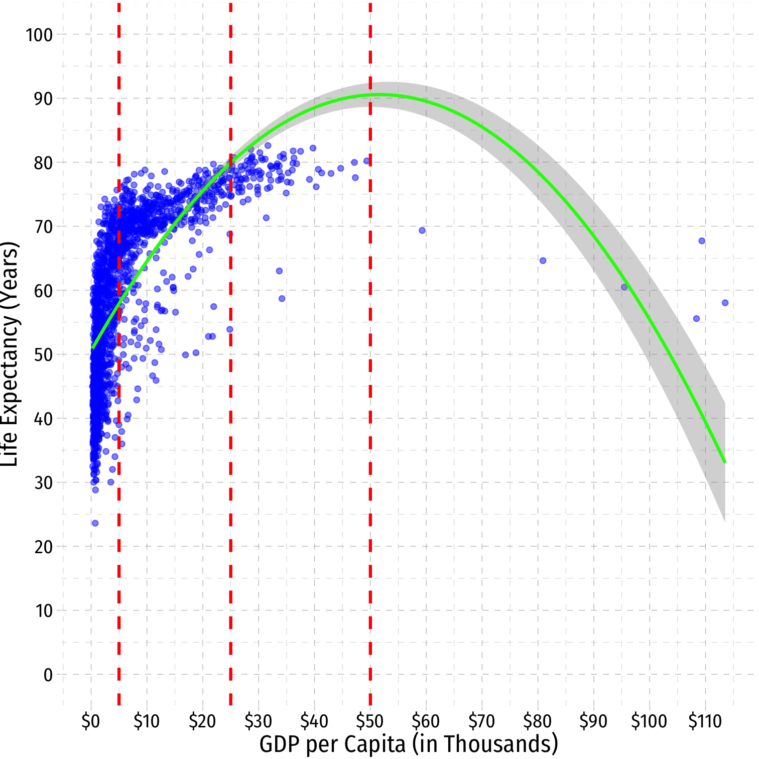
The Quadratic Model: Maxima and Minima
Quadratic Model: Maxima and Minima I
- For a polynomial model, we can also find the predicted maximum or minimum of ^Yi
Quadratic Model: Maxima and Minima I
For a polynomial model, we can also find the predicted maximum or minimum of ^Yi
A quadratic model has a single global maximum or minimum (1 bend)
Quadratic Model: Maxima and Minima I
For a polynomial model, we can also find the predicted maximum or minimum of ^Yi
A quadratic model has a single global maximum or minimum (1 bend)
By calculus, a minimum or maximum occurs where:
∂Yi∂Xi=0β1+2β2Xi=02β2Xi=−β1X∗i=−β12β2
Quadratic Model: Maxima and Minima II
| ABCDEFGHIJ0123456789 |
term <chr> | estimate <dbl> | std.error <dbl> | |
|---|---|---|---|
| (Intercept) | 50.52400578 | 0.2978134673 | |
| GDP_t | 1.55099112 | 0.0373734945 | |
| GDP_sq | -0.01501927 | 0.0005794139 |
Quadratic Model: Maxima and Minima II
| ABCDEFGHIJ0123456789 |
term <chr> | estimate <dbl> | std.error <dbl> | |
|---|---|---|---|
| (Intercept) | 50.52400578 | 0.2978134673 | |
| GDP_t | 1.55099112 | 0.0373734945 | |
| GDP_sq | -0.01501927 | 0.0005794139 |
GDP∗i=−β12β2GDP∗i=−(1.55)2(−0.015)GDP∗i≈51.67
Quadratic Model: Maxima and Minima III
ggplot(data = gapminder)+ aes(x = GDP_t, y = lifeExp)+ geom_point(color="blue", alpha=0.5)+ stat_smooth(method = "lm", formula = y ~ x + I(x^2), color="green")+ geom_vline(xintercept=51.67, linetype="dashed", color="red", size = 1)+ geom_label(x=51.67, y=90, label="$51.67", color="red")+ scale_x_continuous(labels=scales::dollar, breaks=seq(0,120,10))+ scale_y_continuous(breaks=seq(0,100,10), limits=c(0,100))+ labs(x = "GDP per Capita (in Thousands)", y = "Life Expectancy (Years)")+ ggthemes::theme_pander(base_family = "Fira Sans Condensed", base_size=16)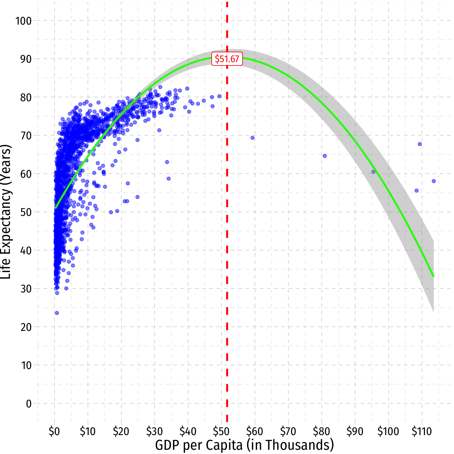
Are Polynomials Necessary?
Determining Polynomials are Necessary I
| ABCDEFGHIJ0123456789 |
term <chr> | estimate <dbl> | std.error <dbl> | statistic <dbl> | p.value <dbl> |
|---|---|---|---|---|
| (Intercept) | 50.52400578 | 0.2978134673 | 169.64984 | 0.000000e+00 |
| GDP_t | 1.55099112 | 0.0373734945 | 41.49976 | 1.292863e-260 |
| GDP_sq | -0.01501927 | 0.0005794139 | -25.92149 | 3.935809e-125 |
- Is the quadratic term necessary?
- Determine if ^β2 (on X2i) is statistically significant:
- H0:^β2=0
- Ha:^β2≠0
- Statistically significant ⟹ we should keep the quadratic model
- If we only ran a linear model, it would be incorrect!
Determining Polynomials are Necessary II
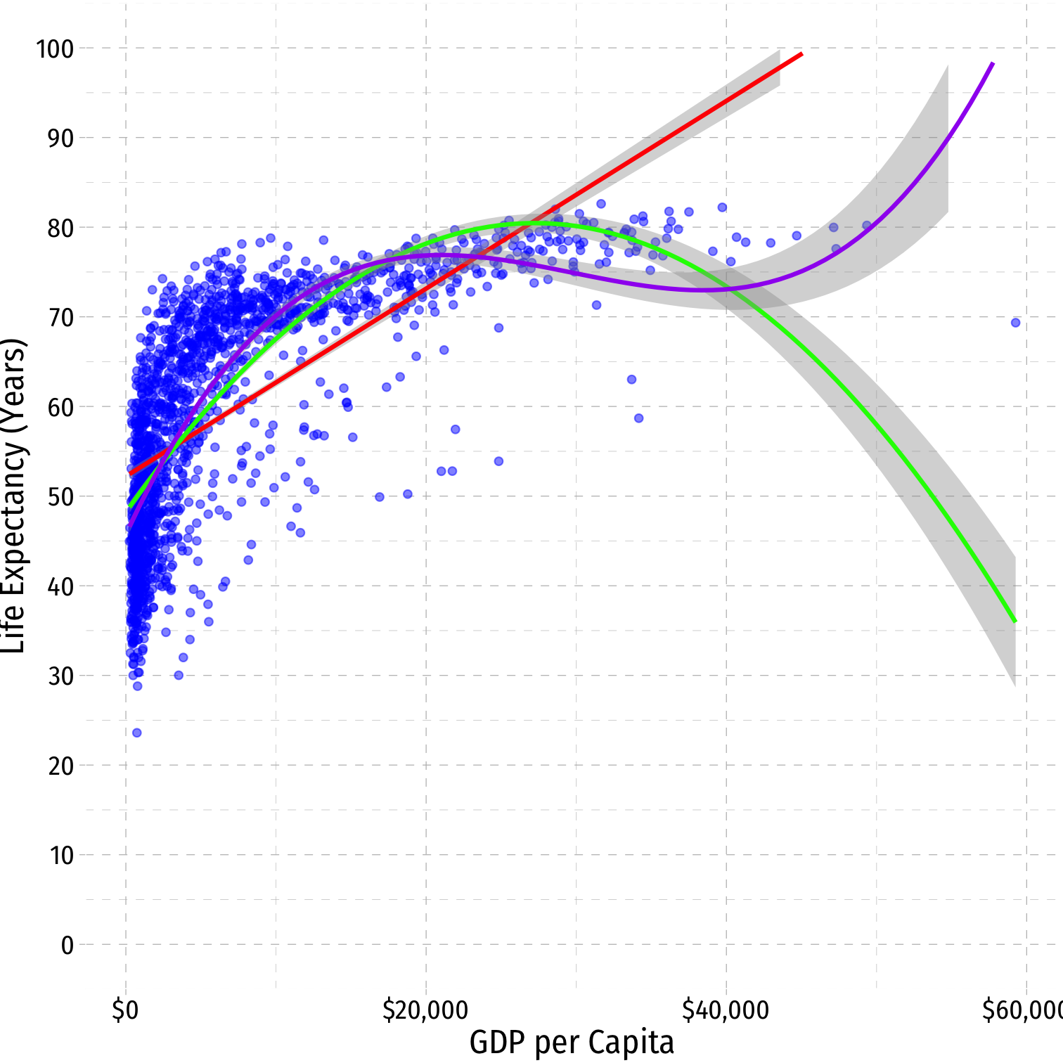
- Should we keep going up in polynomials?
^Life Expectancyi=^β0+^β1GDPi+^β2GDP2i+^β3GDP3i
Determining Polynomials are Necessary III
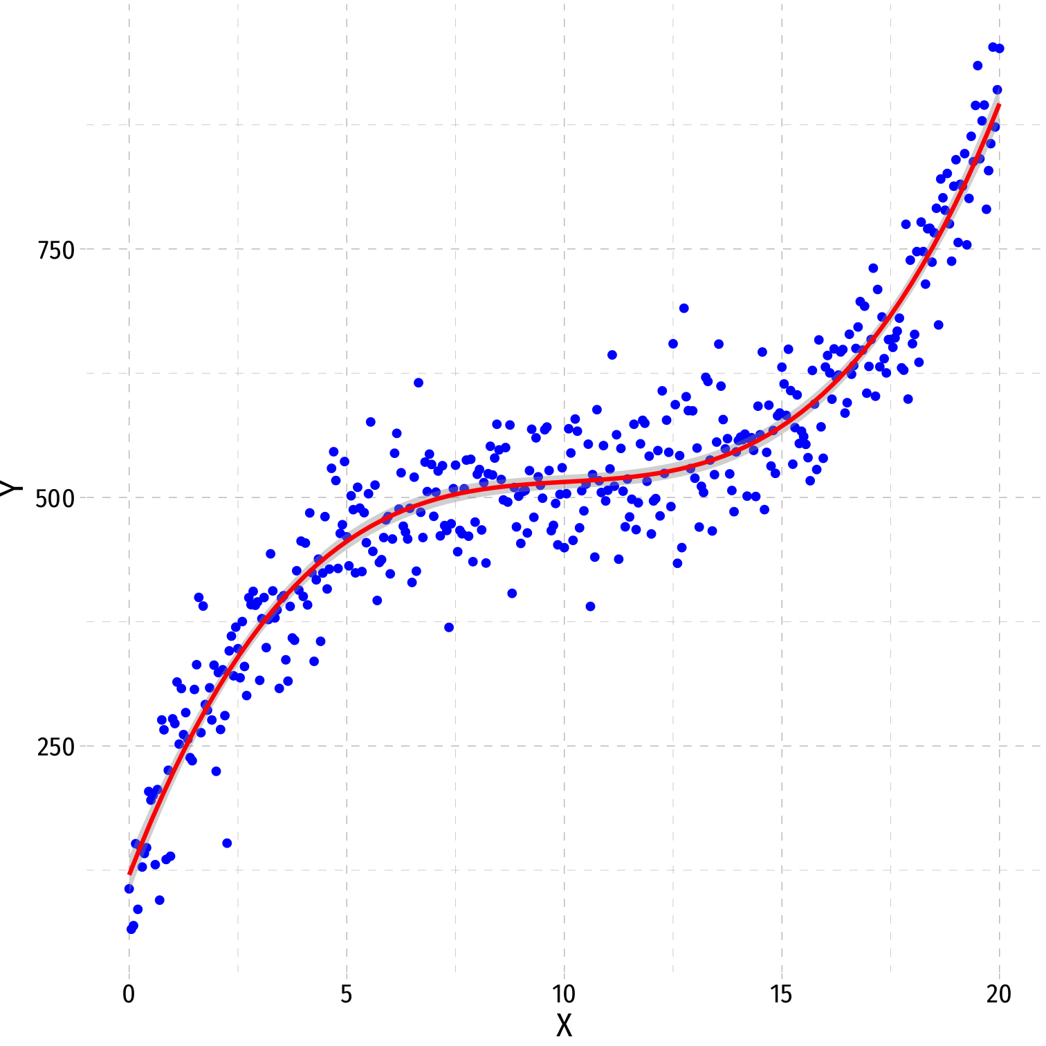
In general, you should have a compelling theoretical reason why data or relationships should “change direction” multiple times
Or clear data patterns that have multiple “bends”
Recall, we care more about accurately measuring the causal effect between X and Y, rather than getting the most accurate prediction possible for ˆY
A Second Polynomial Example I
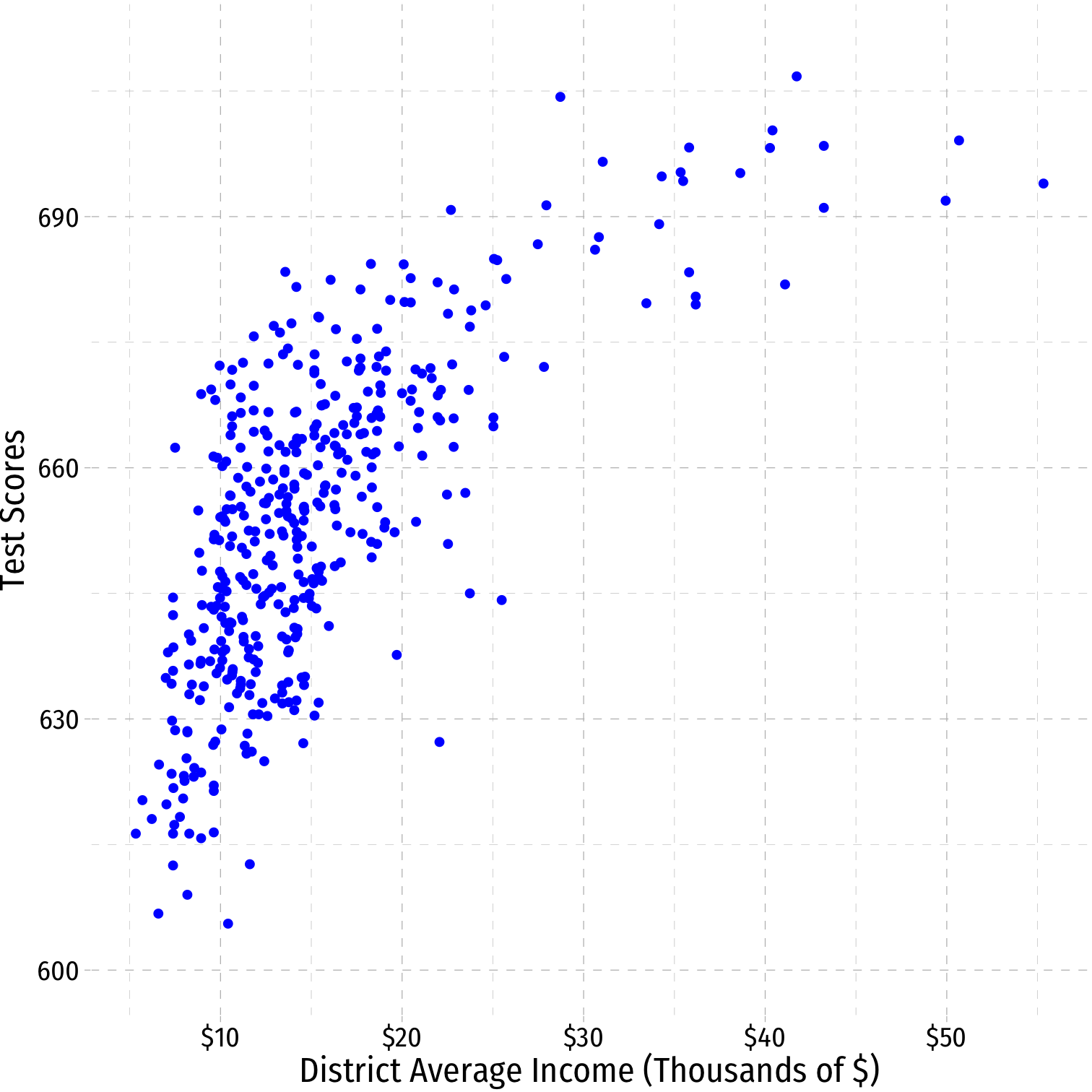
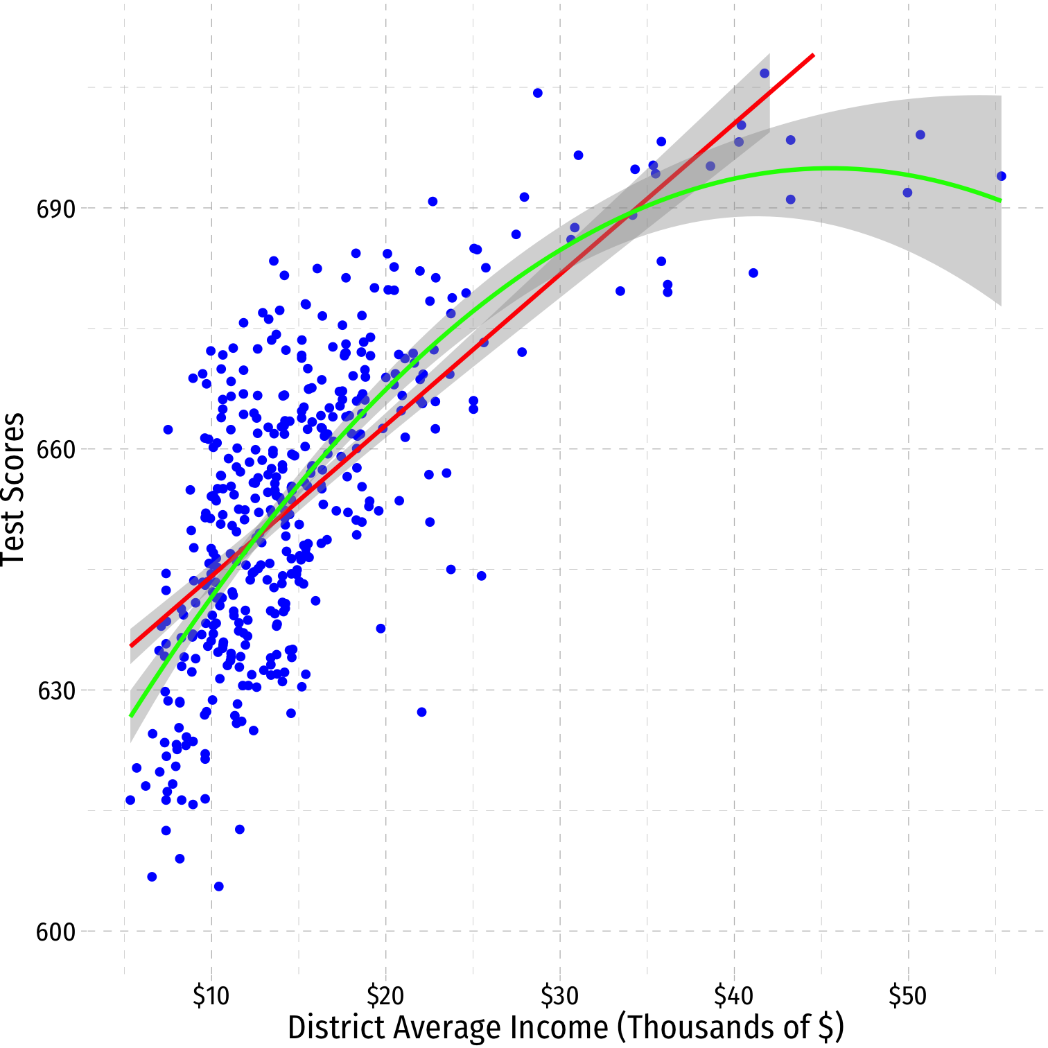
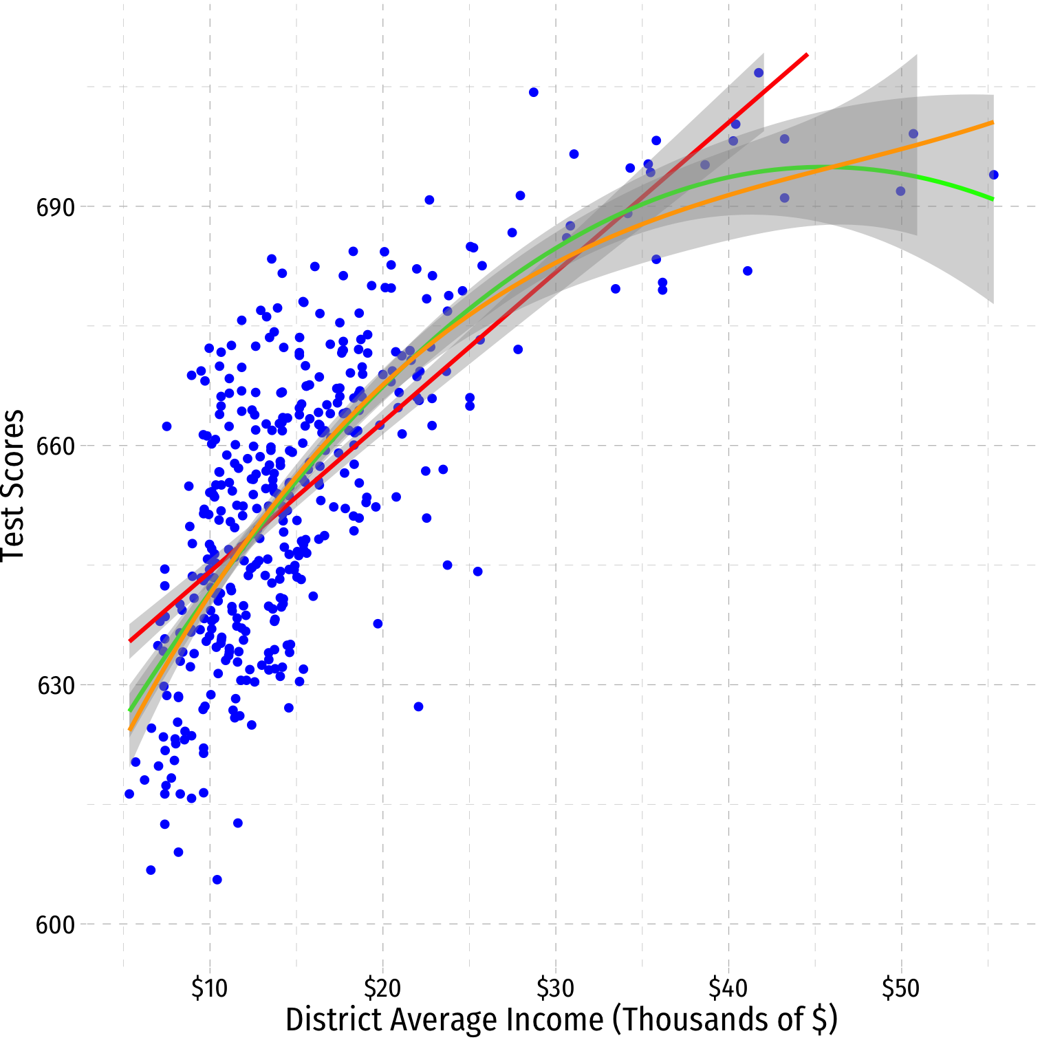
Example: How does a school district's average income affect Test scores?
A Second Polynomial Example I
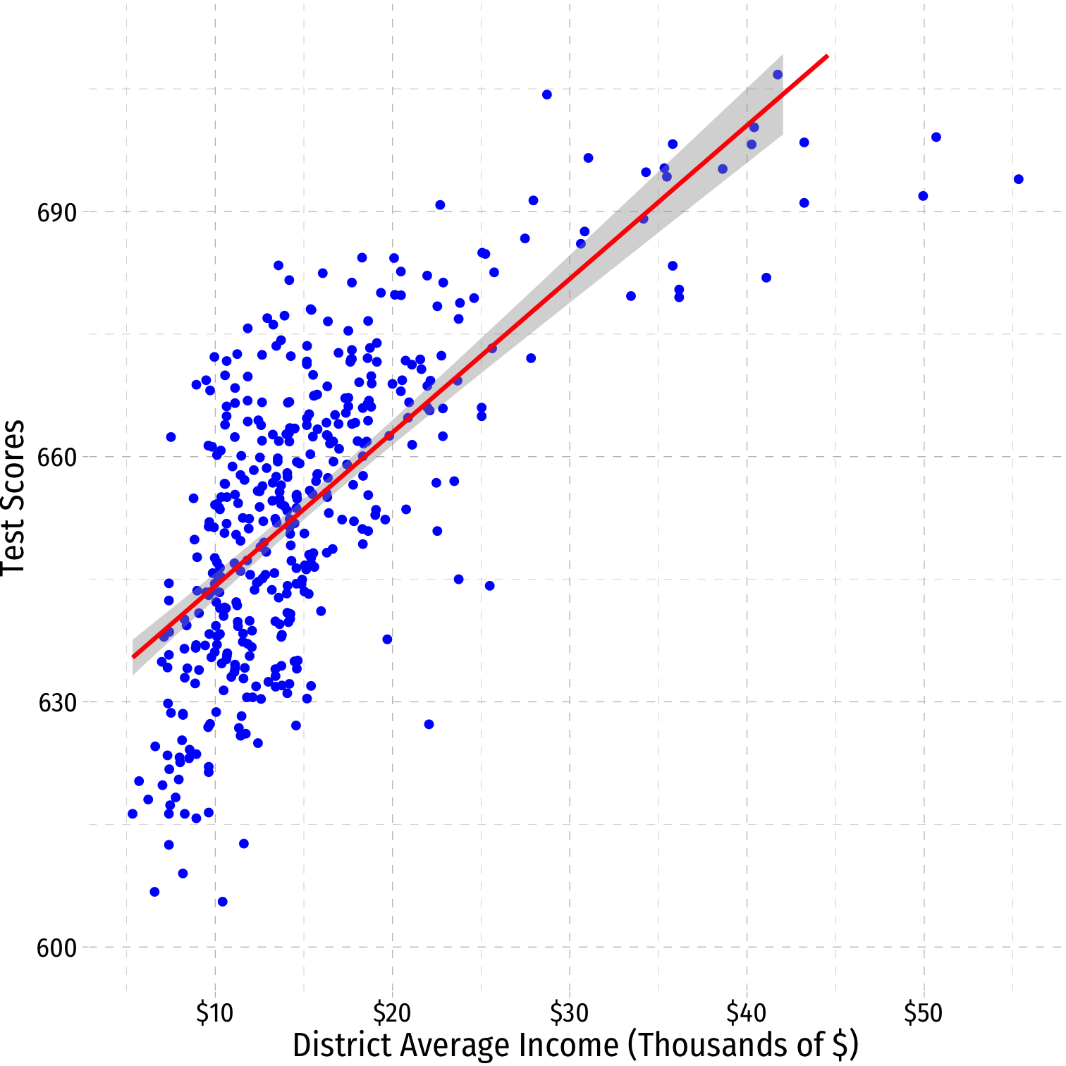
Example: How does a school district's average income affect Test scores?
^Test Scorei=^β0+^β1Incomei
A Second Polynomial Example I
Example: How does a school district's average income affect Test scores?
^Test Scorei=^β0+^β1Incomei+^β1Income2i

A Second Polynomial Example II
| ABCDEFGHIJ0123456789 |
term <chr> | estimate <dbl> | std.error <dbl> | statistic <dbl> | |
|---|---|---|---|---|
| (Intercept) | 607.30173501 | 3.046219282 | 199.362449 | |
| avginc | 3.85099474 | 0.304261693 | 12.656850 | |
| I(avginc^2) | -0.04230846 | 0.006260061 | -6.758474 |
A Second Polynomial Example III
| ABCDEFGHIJ0123456789 |
term <chr> | estimate <dbl> | std.error <dbl> | |
|---|---|---|---|
| (Intercept) | 6.000790e+02 | 5.8295880342 | |
| avginc | 5.018677e+00 | 0.8594537744 | |
| I(avginc^2) | -9.580515e-02 | 0.0373591998 | |
| I(avginc^3) | 6.854842e-04 | 0.0004719549 |
- Should we keep going?
Strategy for Polynomial Model Specification
- Are there good theoretical reasons for relationships changing (e.g. increasing/decreasing returns)?
Strategy for Polynomial Model Specification
Are there good theoretical reasons for relationships changing (e.g. increasing/decreasing returns)?
Plot your data: does a straight line fit well enough?
Strategy for Polynomial Model Specification
Are there good theoretical reasons for relationships changing (e.g. increasing/decreasing returns)?
Plot your data: does a straight line fit well enough?
Specify a polynomial function of a higher power (start with 2) and estimate OLS regression
Strategy for Polynomial Model Specification
Are there good theoretical reasons for relationships changing (e.g. increasing/decreasing returns)?
Plot your data: does a straight line fit well enough?
Specify a polynomial function of a higher power (start with 2) and estimate OLS regression
Use t-test to determine if higher-power term is significant
Interpret effect of change in X on Y
Repeat steps 3-5 as necessary