3.6 — Regression with Categorical Data
ECON 480 • Econometrics • Fall 2021
Ryan Safner
Assistant Professor of Economics
safner@hood.edu
ryansafner/metricsF21
metricsF21.classes.ryansafner.com
Categorical Data
Categorical data place an individual into one of several possible categories
- e.g. sex, season, political party
- may be responses to survey questions
- can be quantitative (e.g. age, zip code)
Rcalls thesefactors

Working with factor Variables in R
Factors in R
factoris a special type ofcharacterobject class that indicates membership in a category (called alevel)Suppose I have data on students:
students %>% head(n = 5)| ABCDEFGHIJ0123456789 |
ID <dbl> | Rank <chr> | Grade <dbl> | ||
|---|---|---|---|---|
| 1 | Sophomore | 77 | ||
| 2 | Senior | 72 | ||
| 3 | Freshman | 73 | ||
| 4 | Senior | 73 | ||
| 5 | Junior | 84 |
- See that
Rankis acharacter(<chr>) variable, just a string of text
Factors in R
- We can make
Rankafactorvariable, to indicate a student is a member of one of the possible categories: (freshman, sophomore, junior, senior)
students <- students %>% mutate(Rank = as.factor(Rank)) # overwrite and change class of Rank to factorstudents %>% head(n = 5)| ABCDEFGHIJ0123456789 |
ID <dbl> | Rank <fct> | Grade <dbl> | ||
|---|---|---|---|---|
| 1 | Sophomore | 77 | ||
| 2 | Senior | 72 | ||
| 3 | Freshman | 73 | ||
| 4 | Senior | 73 | ||
| 5 | Junior | 84 |
- See now it’s a
factor(<fct>)
Factors in R
# what are the categories?students %>% group_by(Rank) %>% count()| ABCDEFGHIJ0123456789 |
Rank <fct> | n <int> | |||
|---|---|---|---|---|
| Freshman | 1 | |||
| Junior | 4 | |||
| Senior | 2 | |||
| Sophomore | 3 |
# note the order is arbitrary! This is an "unordered" factorOrdered Factors in R
- If there is a rank order you wish to preserve, you can make an
ordered(factor) variable- list the
levelsfrom 1st to last
- list the
students <- students %>% mutate(Rank = ordered(Rank, # overwrite and change class of Rank to ordered # next, specify the levels, in order levels = c("Freshman", "Sophomore", "Junior", "Senior") ) )students %>% head(n = 5)| ABCDEFGHIJ0123456789 |
ID <dbl> | Rank <ord> | Grade <dbl> | ||
|---|---|---|---|---|
| 1 | Sophomore | 77 | ||
| 2 | Senior | 72 | ||
| 3 | Freshman | 73 | ||
| 4 | Senior | 73 | ||
| 5 | Junior | 84 |
Ordered Factors in R
students %>% group_by(Rank) %>% count()| ABCDEFGHIJ0123456789 |
Rank <ord> | n <int> | |||
|---|---|---|---|---|
| Freshman | 1 | |||
| Sophomore | 3 | |||
| Junior | 4 | |||
| Senior | 2 |
Example Research Question
Example: How much higher wages, on average, do men earn compared to women?

The Pure Statistics of Comparing Group Means
Basic statistics: can test for statistically significant difference in group means with a t-test†, let:
YM: average earnings of a sample of nM men
YW: average earnings of a sample of nW women
Difference in group averages: d= ˉYM − ˉYW
The hypothesis test is:
- H0:d=0
- H1:d≠0
† See today’s class page for this example
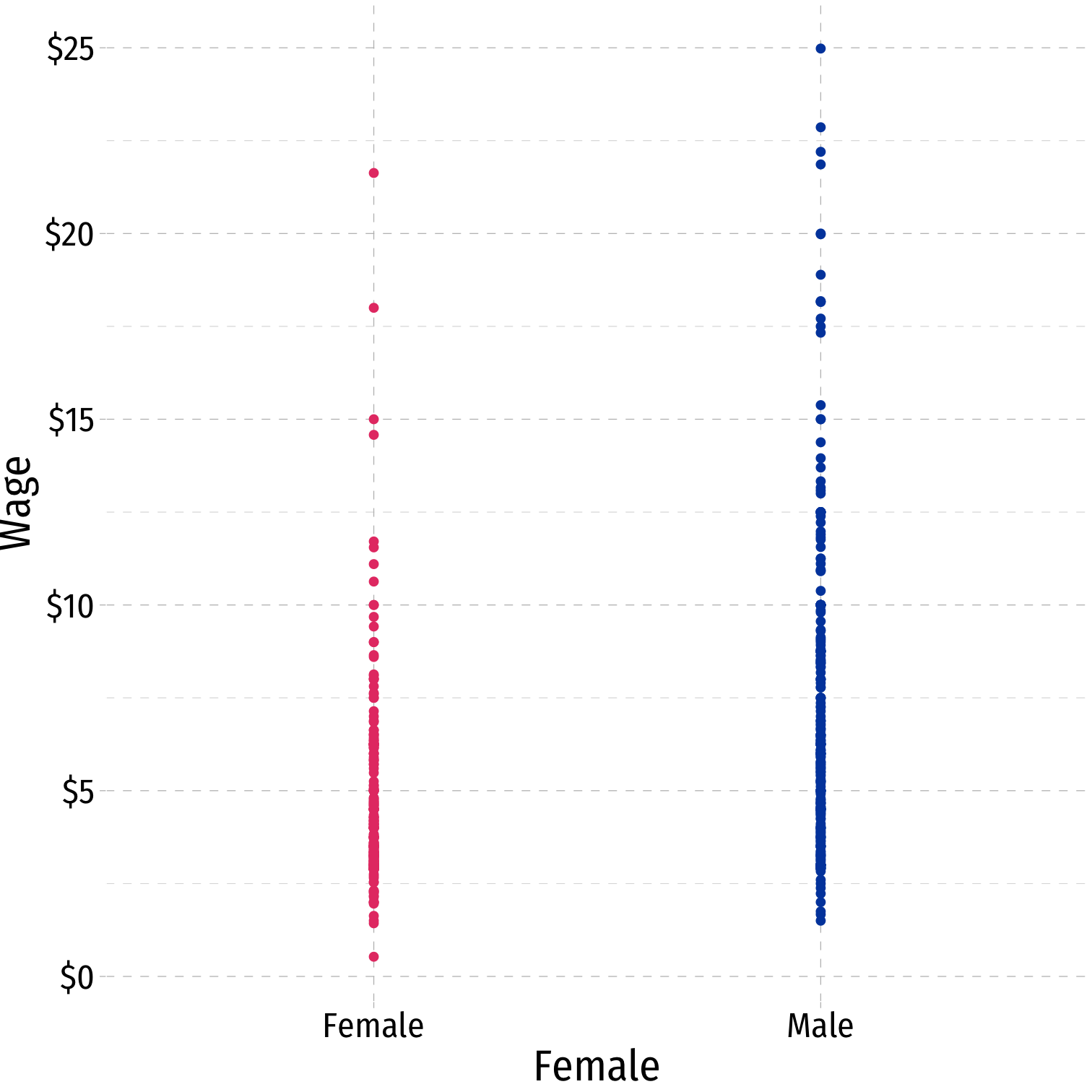
Plotting Factors in R
If I plot a
factorvariable, e.g.Gender(which is eitherMaleorFemale), the scatterplot withwagelooks like this- effectively
Rtreats values of a factor variable as integers - in this case,
"Female"= 0,"Male"= 1
- effectively
Let’s make this more explicit by making a dummy variable to stand in for Gender
Regression with Dummy Variables
Comparing Groups with Regression
In a regression, we can easily compare across groups via a dummy variable†
Dummy variable only =0 or =1, if a condition is
TRUEvs.FALSESignifies whether an observation belongs to a category or not
† Also called a binary variable or dichotomous variable
Comparing Groups with Regression
In a regression, we can easily compare across groups via a dummy variable†
Dummy variable only =0 or =1, if a condition is
TRUEvs.FALSESignifies whether an observation belongs to a category or not
† Also called a binary variable or dichotomous variable
Example:
^Wagei=^β0+^β1Femalei where Femalei={1if individual i is Female0if individual i is Male
- Again, ^β1 makes less sense as the “slope” of a line in this context
Comparing Groups in Regression: Scatterplot
Femaleis our dummy x-variableHard to see relationships because of overplotting
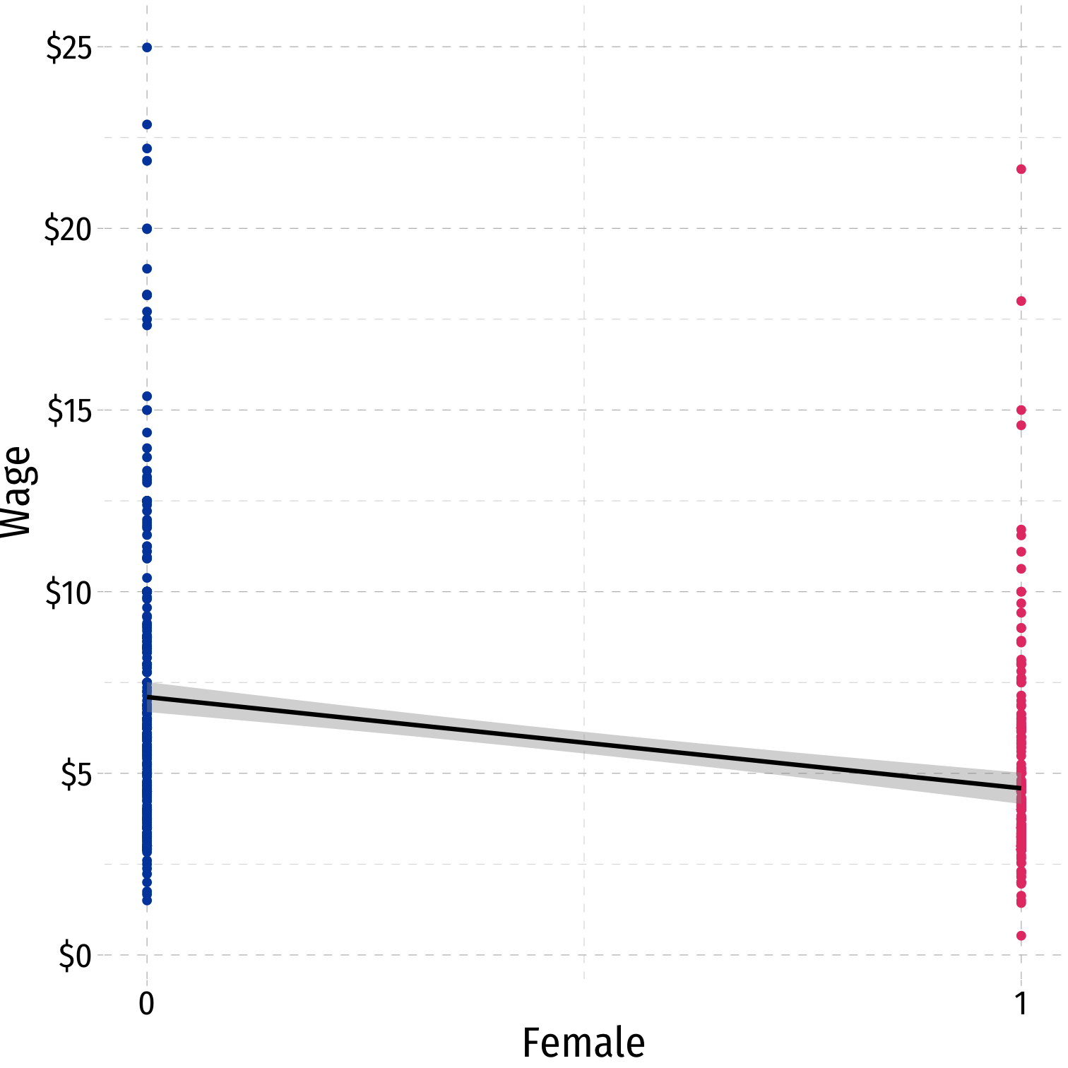
Comparing Groups in Regression: Scatterplot
Femaleis our dummy x-variableHard to see relationships because of overplotting
Tip: use
geom_jitter()instead ofgeom_point()to randomly nudge points to see them better!- Only used for plotting, does not affect actual data, regression, etc.
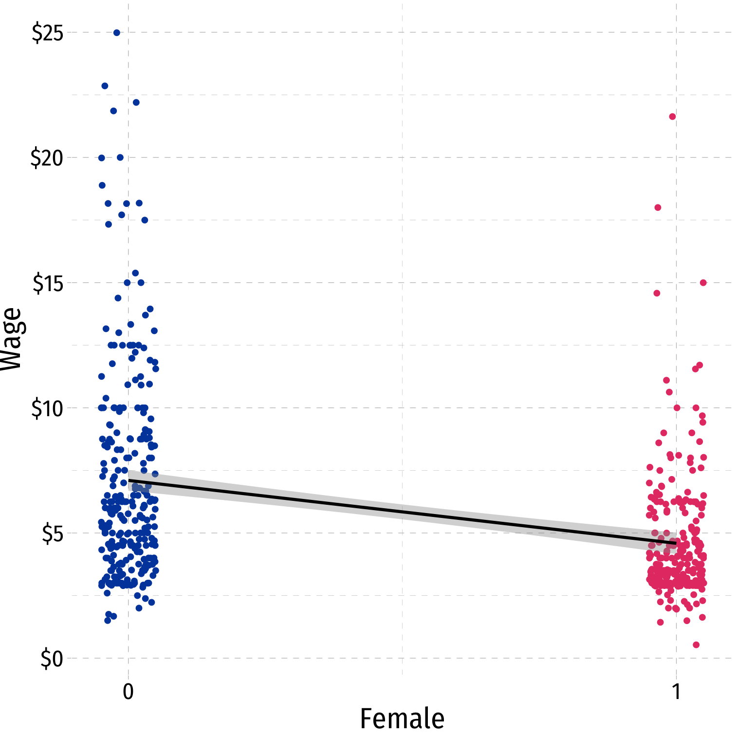
Comparing Groups in Regression: Scatterplot
Femaleis our dummy x-variableHard to see relationships because of overplotting
Use
geom_jitter()instead ofgeom_point()to randomly nudge points- Only for plotting purposes, does not affect actual data, regression, etc.
Dummy Variables as Group Means
^Yi=^β0+^β1Di where Di={0,1}
Dummy Variables as Group Means
^Yi=^β0+^β1Di where Di={0,1}
- When Di=0 (“Control group”):
- ^Yi=^β0
- E[Yi|Di=0]=^β0 ⟺ the mean of Y when Di=0
Dummy Variables as Group Means
^Yi=^β0+^β1Di where Di={0,1}
- When Di=0 (“Control group”):
- ^Yi=^β0
- E[Yi|Di=0]=^β0 ⟺ the mean of Y when Di=0
- When Di=1 (“Treatment group”):
- ^Yi=^β0+^β1Di
- E[Yi|Di=1]=^β0+^β1 ⟺ the mean of Y when Di=1
Dummy Variables as Group Means
^Yi=^β0+^β1Di where Di={0,1}
- When Di=0 (“Control group”):
- ^Yi=^β0
- E[Yi|Di=0]=^β0 ⟺ the mean of Y when Di=0
- When Di=1 (“Treatment group”):
- ^Yi=^β0+^β1Di
- E[Yi|Di=1]=^β0+^β1 ⟺ the mean of Y when Di=1
- So the difference in group means:
=E[Yi|Di=1]−E[Yi|Di=0]=(^β0+^β1)−(^β0)=^β1
Dummy Variables as Group Means: Our Example
Example:
^Wagei=^β0+^β1Femalei
where Femalei={1if i is Female0if i is Male
- Mean wage for men:
Dummy Variables as Group Means: Our Example
Example:
^Wagei=^β0+^β1Femalei
where Femalei={1if i is Female0if i is Male
- Mean wage for men:
E[Wage|Female=0]=^β0
Dummy Variables as Group Means: Our Example
Example:
^Wagei=^β0+^β1Femalei
where Femalei={1if i is Female0if i is Male
Mean wage for men: E[Wage|Female=0]=^β0
Mean wage for women:
Dummy Variables as Group Means: Our Example
Example:
^Wagei=^β0+^β1Femalei
where Femalei={1if i is Female0if i is Male
Mean wage for men: E[Wage|Female=0]=^β0
Mean wage for women: E[Wage|Female=1]=^β0+^β1
Dummy Variables as Group Means: Our Example
Example:
^Wagei=^β0+^β1Femalei
where Femalei={1if i is Female0if i is Male
Mean wage for men: E[Wage|Female=0]=^β0
Mean wage for women: E[Wage|Female=1]=^β0+^β1
Difference in wage between men & women:
Dummy Variables as Group Means: Our Example
Example:
^Wagei=^β0+^β1Femalei
where Femalei={1if i is Female0if i is Male
Mean wage for men: E[Wage|Female=0]=^β0
Mean wage for women: E[Wage|Female=1]=^β0+^β1
Difference in wage between men & women: ^β1
Comparing Groups in Regression: Scatterplot
^Wagei=^β0+^β1Femalei
where Femalei={1if i is Female0if i is Male
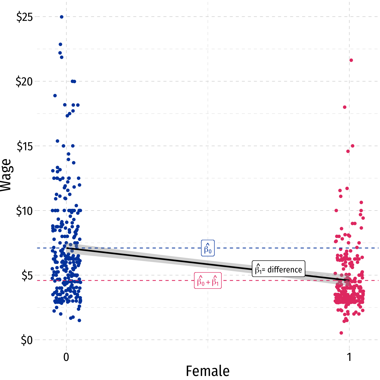
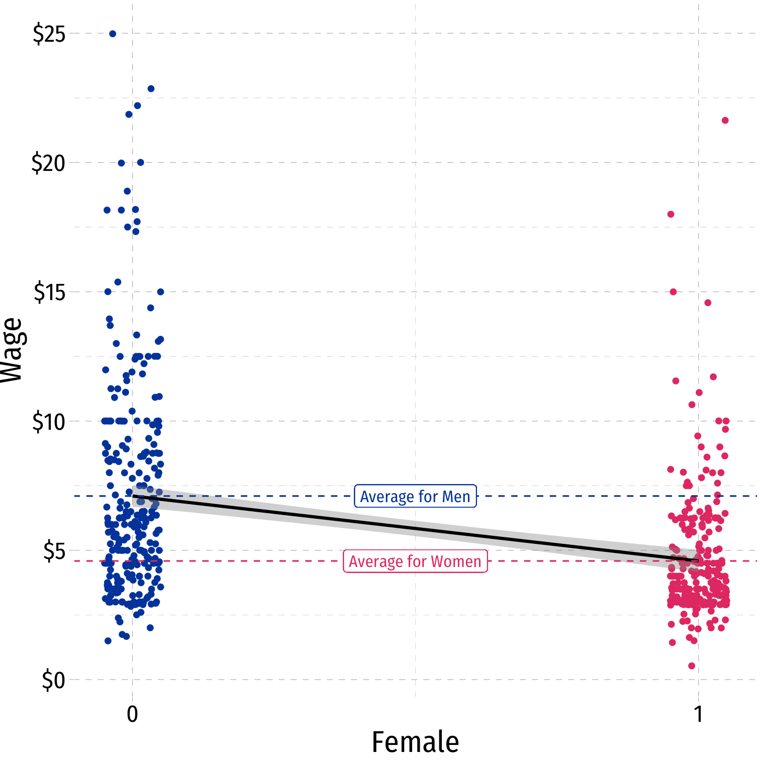
The Data
# comes from wooldridge package# install.packages("wooldridge")library(wooldridge)# data is called "wage1", save as a dataframe I'll call "wages"wages <- wage1wages %>% head()Get Group Averages & Std. Devs.
# Summarize for Menwages %>% filter(female==0) %>% summarize(mean = mean(wage), sd = sd(wage))| ABCDEFGHIJ0123456789 |
mean <dbl> | sd <dbl> | |
|---|---|---|
| 7.099489 | 4.160858 |
# Summarize for Womenwages %>% filter(female==1) %>% summarize(mean = mean(wage), sd = sd(wage))| ABCDEFGHIJ0123456789 |
mean <dbl> | sd <dbl> | |
|---|---|---|
| 4.587659 | 2.529363 |
Visualize Differences
The Regression I
femalereg <- lm(wage ~ female, data = wages)summary(femalereg)## ## Call:## lm(formula = wage ~ female, data = wages)## ## Residuals:## Min 1Q Median 3Q Max ## -5.5995 -1.8495 -0.9877 1.4260 17.8805 ## ## Coefficients:## Estimate Std. Error t value Pr(>|t|) ## (Intercept) 7.0995 0.2100 33.806 < 2e-16 ***## female -2.5118 0.3034 -8.279 1.04e-15 ***## ---## Signif. codes: 0 '***' 0.001 '**' 0.01 '*' 0.05 '.' 0.1 ' ' 1## ## Residual standard error: 3.476 on 524 degrees of freedom## Multiple R-squared: 0.1157, Adjusted R-squared: 0.114 ## F-statistic: 68.54 on 1 and 524 DF, p-value: 1.042e-15The Regression I
femalereg <- lm(wage ~ female, data = wages)summary(femalereg)## ## Call:## lm(formula = wage ~ female, data = wages)## ## Residuals:## Min 1Q Median 3Q Max ## -5.5995 -1.8495 -0.9877 1.4260 17.8805 ## ## Coefficients:## Estimate Std. Error t value Pr(>|t|) ## (Intercept) 7.0995 0.2100 33.806 < 2e-16 ***## female -2.5118 0.3034 -8.279 1.04e-15 ***## ---## Signif. codes: 0 '***' 0.001 '**' 0.01 '*' 0.05 '.' 0.1 ' ' 1## ## Residual standard error: 3.476 on 524 degrees of freedom## Multiple R-squared: 0.1157, Adjusted R-squared: 0.114 ## F-statistic: 68.54 on 1 and 524 DF, p-value: 1.042e-15library(broom)tidy(femalereg)| ABCDEFGHIJ0123456789 |
term <chr> | estimate <dbl> | std.error <dbl> | statistic <dbl> | |
|---|---|---|---|---|
| (Intercept) | 7.099489 | 0.2100082 | 33.805777 | |
| female | -2.511830 | 0.3034092 | -8.278688 |
Dummy Regression vs. Group Means
From tabulation of group means
| Gender | Avg. Wage | Std. Dev. | n |
|---|---|---|---|
| Female | 4.59 | 2.33 | 252 |
| Male | 7.10 | 4.16 | 274 |
| Difference | 2.51 | 0.30 | − |
From t-test of difference in group means
| ABCDEFGHIJ0123456789 |
term <chr> | estimate <dbl> | std.error <dbl> | |
|---|---|---|---|
| (Intercept) | 7.099489 | 0.2100082 | |
| female | -2.511830 | 0.3034092 |
^Wagesi=7.10−2.51Femalei
Recoding Dummies
Recoding Dummies
Example:
- Suppose instead of female we had used:
^Wagei=^β0+^β1Malei where Malei={1if person i is Male0if person i is Female
Recoding Dummies with Data
wages<-wages %>% mutate(male = ifelse(female == 0, # condition: is female equal to 0? yes = 1, # if true: code as "1" no = 0)) # if false: code as "0"# verify it workedwages %>% select(wage, female, male) %>% head()| ABCDEFGHIJ0123456789 |
wage <dbl> | female <int> | male <dbl> | ||
|---|---|---|---|---|
| 1 | 3.10 | 1 | 0 | |
| 2 | 3.24 | 1 | 0 | |
| 3 | 3.00 | 0 | 1 | |
| 4 | 6.00 | 0 | 1 | |
| 5 | 5.30 | 0 | 1 | |
| 6 | 8.75 | 0 | 1 |
Scatterplot with Male

Scatterplot with Male
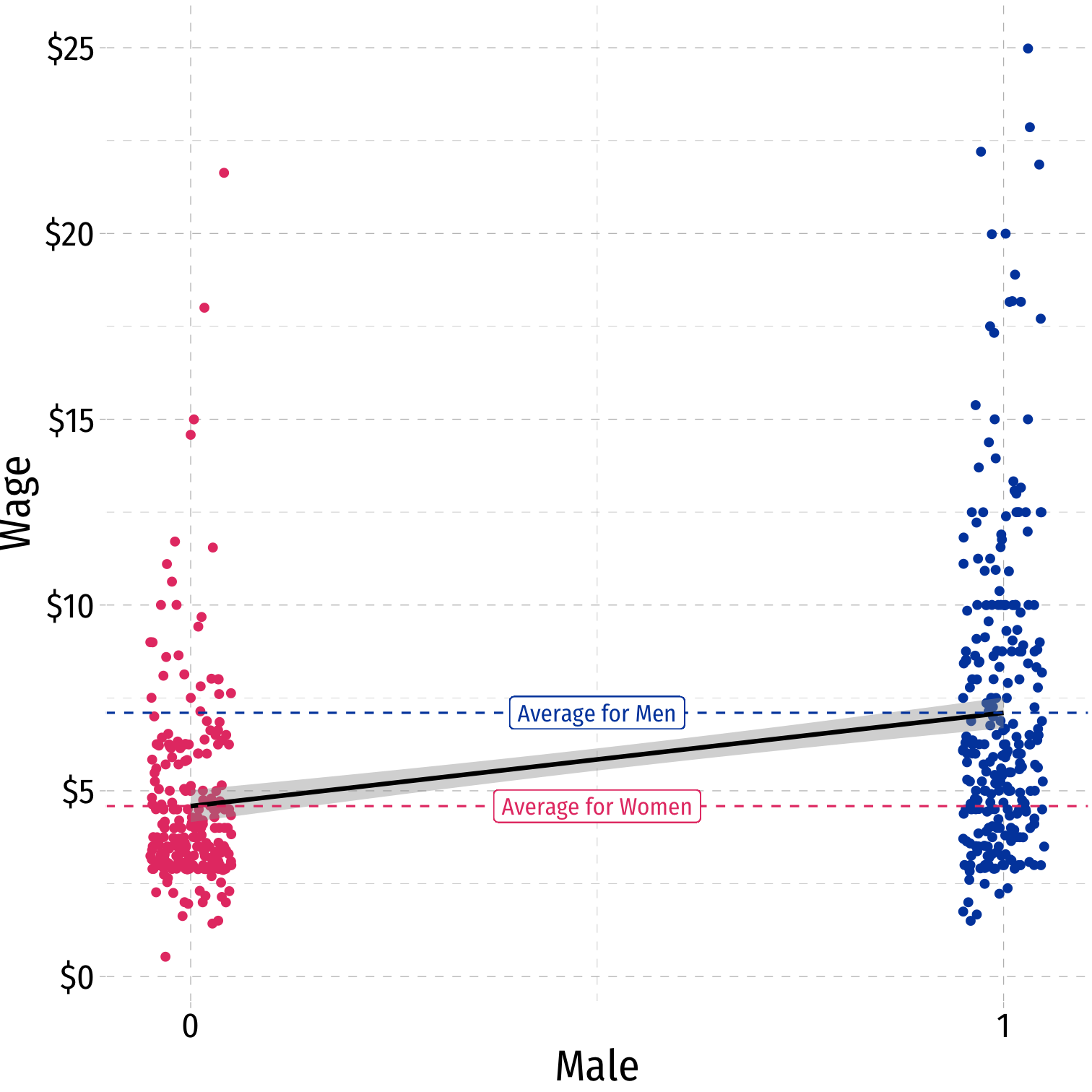
Dummy Variables as Group Means: With Male
Example:
^Wagei=^β0+^β1Malei
where Malei={1if i is Male0if i is Female
Mean wage for men: E[Wage|Male=1]=^β0+^β1
Mean wage for women: E[Wage|Male=0]=^β0
Difference in wage between men & women: ^β1
Scatterplot with Male

Scatterplot with Male
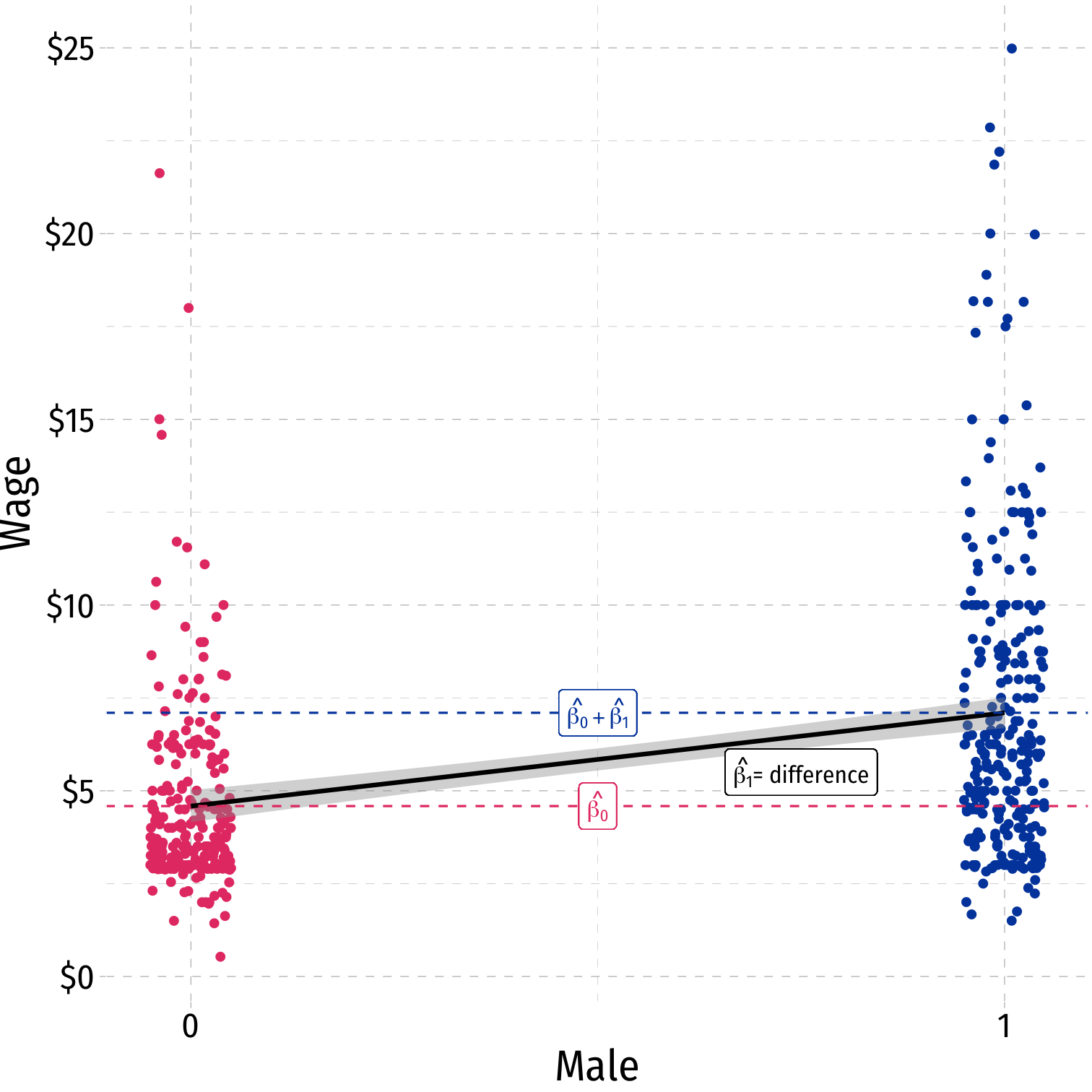
The Regression with Male I
malereg <- lm(wage ~ male, data = wages)summary(malereg)## ## Call:## lm(formula = wage ~ male, data = wages)## ## Residuals:## Min 1Q Median 3Q Max ## -5.5995 -1.8495 -0.9877 1.4260 17.8805 ## ## Coefficients:## Estimate Std. Error t value Pr(>|t|) ## (Intercept) 4.5877 0.2190 20.950 < 2e-16 ***## male 2.5118 0.3034 8.279 1.04e-15 ***## ---## Signif. codes: 0 '***' 0.001 '**' 0.01 '*' 0.05 '.' 0.1 ' ' 1## ## Residual standard error: 3.476 on 524 degrees of freedom## Multiple R-squared: 0.1157, Adjusted R-squared: 0.114 ## F-statistic: 68.54 on 1 and 524 DF, p-value: 1.042e-15The Regression with Male I
malereg <- lm(wage ~ male, data = wages)summary(malereg)## ## Call:## lm(formula = wage ~ male, data = wages)## ## Residuals:## Min 1Q Median 3Q Max ## -5.5995 -1.8495 -0.9877 1.4260 17.8805 ## ## Coefficients:## Estimate Std. Error t value Pr(>|t|) ## (Intercept) 4.5877 0.2190 20.950 < 2e-16 ***## male 2.5118 0.3034 8.279 1.04e-15 ***## ---## Signif. codes: 0 '***' 0.001 '**' 0.01 '*' 0.05 '.' 0.1 ' ' 1## ## Residual standard error: 3.476 on 524 degrees of freedom## Multiple R-squared: 0.1157, Adjusted R-squared: 0.114 ## F-statistic: 68.54 on 1 and 524 DF, p-value: 1.042e-15library(broom)tidy(malereg)| ABCDEFGHIJ0123456789 |
term <chr> | estimate <dbl> | std.error <dbl> | statistic <dbl> | |
|---|---|---|---|---|
| (Intercept) | 4.587659 | 0.2189834 | 20.949802 | |
| male | 2.511830 | 0.3034092 | 8.278688 |
The Dummy Regression: Male or Female
| (1) | (2) | |
|---|---|---|
| Constant | 4.59 *** | 7.10 *** |
| (0.22) | (0.21) | |
| Female | -2.51 *** | |
| (0.30) | ||
| Male | 2.51 *** | |
| (0.30) | ||
| N | 526 | 526 |
| R-Squared | 0.12 | 0.12 |
| SER | 3.48 | 3.48 |
| *** p < 0.001; ** p < 0.01; * p < 0.05. | ||
Note it doesn't matter if we use
maleorfemale, males always earn $2.51 more than femalesCompare the constant (average for the D=0 group)
Should you use
maleANDfemale? We'll come to that...
Categorical Variables (More than 2 Categories)
Categorical Variables with More than 2 Categories
- A categorical variable expresses membership in a category, where there is no ranking or hierarchy of the categories
- We've looked at categorical variables with 2 categories only
- e.g. Male/Female, Spring/Summer/Fall/Winter, Democratic/Republican/Independent
- Might be an ordinal variable expresses rank or an ordering of data, but not necessarily their relative magnitude
- e.g. Order of finalists in a competition (1st, 2nd, 3rd)
- e.g. Highest education attained (1=elementary school, 2=high school, 3=bachelor's degree, 4=graduate degree)
Using Categorical Variables in Regression I
Example: How do wages vary by region of the country? Let Regioni={Northeast,Midwest,South,West}
Using Categorical Variables in Regression I
Example: How do wages vary by region of the country? Let Regioni={Northeast,Midwest,South,West}
- Can we run the following regression?
^Wagesi=^β0+^β1Regioni
Using Categorical Variables in Regression II
Example: How do wages vary by region of the country?
Code region numerically: Regioni={1if i is in Northeast2if i is in Midwest3if i is in South4if i is in West
Using Categorical Variables in Regression II
Example: How do wages vary by region of the country?
Code region numerically: Regioni={1if i is in Northeast2if i is in Midwest3if i is in South4if i is in West
- Can we run the following regression?
^Wagesi=^β0+^β1Regioni
Using Categorical Variables in Regression III
Example: How do wages vary by region of the country?
Create a dummy variable for each region:
- Northeasti=1 if i is in Northeast, otherwise =0
- Midwesti=1 if i is in Midwest, otherwise =0
- Southi=1 if i is in South, otherwise =0
- Westi=1 if i is in West, otherwise =0
- Can we run the following regression?
^Wagesi=^β0+^β1Northeasti+^β2Midwesti+^β3Southi+^β4Westi
- For every i:Northeasti+Midwesti+Southi+Westi=1!
The Dummy Variable Trap
Example: ^Wagesi=^β0+^β1Northeasti+^β2Midwesti+^β3Southi+^β4Westi
- If we include all possible categories, they are perfectly multicollinear, an exact linear function of one another:
Northeasti+Midwesti+Southi+Westi=1∀i
- This is known as the dummy variable trap, a common source of perfect multicollinearity
The Reference Category
To avoid the dummy variable trap, always omit one category from the regression, known as the “reference category”
It does not matter which category we omit!
Coefficients on each dummy variable measure the difference between the reference category and each category dummy
The Reference Category: Example
Example: ^Wagesi=^β0+^β1Northeasti+^β2Midwesti+^β3Southi
- Westi is omitted (arbitrarily chosen)
The Reference Category: Example
Example: ^Wagesi=^β0+^β1Northeasti+^β2Midwesti+^β3Southi
Westi is omitted (arbitrarily chosen)
^β0:
The Reference Category: Example
Example: ^Wagesi=^β0+^β1Northeasti+^β2Midwesti+^β3Southi
Westi is omitted (arbitrarily chosen)
^β0: average wage for i in the West
The Reference Category: Example
Example: ^Wagesi=^β0+^β1Northeasti+^β2Midwesti+^β3Southi
Westi is omitted (arbitrarily chosen)
^β0: average wage for i in the West
^β1:
The Reference Category: Example
Example: ^Wagesi=^β0+^β1Northeasti+^β2Midwesti+^β3Southi
Westi is omitted (arbitrarily chosen)
^β0: average wage for i in the West
^β1: difference between West and Northeast
The Reference Category: Example
Example: ^Wagesi=^β0+^β1Northeasti+^β2Midwesti+^β3Southi
Westi is omitted (arbitrarily chosen)
^β0: average wage for i in the West
^β1: difference between West and Northeast
^β2:
The Reference Category: Example
Example: ^Wagesi=^β0+^β1Northeasti+^β2Midwesti+^β3Southi
Westi is omitted (arbitrarily chosen)
^β0: average wage for i in the West
^β1: difference between West and Northeast
^β2: difference between West and Midwest
The Reference Category: Example
Example: ^Wagesi=^β0+^β1Northeasti+^β2Midwesti+^β3Southi
Westi is omitted (arbitrarily chosen)
^β0: average wage for i in the West
^β1: difference between West and Northeast
^β2: difference between West and Midwest
^β3:
The Reference Category: Example
Example: ^Wagesi=^β0+^β1Northeasti+^β2Midwesti+^β3Southi
Westi is omitted (arbitrarily chosen)
^β0: average wage for i in the West
^β1: difference between West and Northeast
^β2: difference between West and Midwest
^β3: difference between West and South
Dummy Variable Trap in R
lm(wage ~ noreast + northcen + south + west, data = wages) %>% summary()## ## Call:## lm(formula = wage ~ noreast + northcen + south + west, data = wages)## ## Residuals:## Min 1Q Median 3Q Max ## -6.083 -2.387 -1.097 1.157 18.610 ## ## Coefficients: (1 not defined because of singularities)## Estimate Std. Error t value Pr(>|t|) ## (Intercept) 6.6134 0.3891 16.995 < 2e-16 ***## noreast -0.2436 0.5154 -0.473 0.63664 ## northcen -0.9029 0.5035 -1.793 0.07352 . ## south -1.2265 0.4728 -2.594 0.00974 ** ## west NA NA NA NA ## ---## Signif. codes: 0 '***' 0.001 '**' 0.01 '*' 0.05 '.' 0.1 ' ' 1## ## Residual standard error: 3.671 on 522 degrees of freedom## Multiple R-squared: 0.0175, Adjusted R-squared: 0.01185 ## F-statistic: 3.099 on 3 and 522 DF, p-value: 0.02646Using Different Reference Categories in R
# let's run 4 regressions, each one we omit a different regionno_noreast_reg <- lm(wage ~ northcen + south + west, data = wages)no_northcen_reg <- lm(wage ~ noreast + south + west, data = wages)no_south_reg <- lm(wage ~ noreast + northcen + west, data = wages)no_west_reg <- lm(wage ~ noreast + northcen + south, data = wages)# now make an output tablelibrary(huxtable)huxreg(no_noreast_reg, no_northcen_reg, no_south_reg, no_west_reg, coefs = c("Constant" = "(Intercept)", "Northeast" = "noreast", "Midwest" = "northcen", "South" = "south", "West" = "west"), statistics = c("N" = "nobs", "R-Squared" = "r.squared", "SER" = "sigma"), number_format = 3)Using Different Reference Categories in R II
| (1) | (2) | (3) | (4) | |
|---|---|---|---|---|
| Constant | 6.370 *** | 5.710 *** | 5.387 *** | 6.613 *** |
| (0.338) | (0.320) | (0.268) | (0.389) | |
| Northeast | 0.659 | 0.983 * | -0.244 | |
| (0.465) | (0.432) | (0.515) | ||
| Midwest | -0.659 | 0.324 | -0.903 | |
| (0.465) | (0.417) | (0.504) | ||
| South | -0.983 * | -0.324 | -1.226 ** | |
| (0.432) | (0.417) | (0.473) | ||
| West | 0.244 | 0.903 | 1.226 ** | |
| (0.515) | (0.504) | (0.473) | ||
| N | 526 | 526 | 526 | 526 |
| R-Squared | 0.017 | 0.017 | 0.017 | 0.017 |
| SER | 3.671 | 3.671 | 3.671 | 3.671 |
| *** p < 0.001; ** p < 0.01; * p < 0.05. | ||||
Constant is alsways average wage for reference (omitted) region
Compare coefficients between Midwest in (1) and Northeast in (2)...
Compare coefficients between West in (3) and South in (4)...
Does not matter which region we omit!
- Same R2, SER, coefficients give same results
Dummy Dependent (Y) Variables
- In many contexts, we will want to have our dependent (Y) variable be a dummy variable
Dummy Dependent (Y) Variables
- In many contexts, we will want to have our dependent (Y) variable be a dummy variable
Example: ^Admittedi=^β0+^β1GPAi where Admittedi={1if i is Admitted0if i is Not Admitted
Dummy Dependent (Y) Variables
- In many contexts, we will want to have our dependent (Y) variable be a dummy variable
Example: ^Admittedi=^β0+^β1GPAi where Admittedi={1if i is Admitted0if i is Not Admitted
- A model where Y is a dummy is called a linear probability model, as it measures the probability of Y occuring (=1) given the X's, i.e. P(Yi=1|X1,⋯,Xk)
- e.g. the probability person i is Admitted to a program with a given GPA
Requires special tools to properly interpret and extend this (logit, probit, etc)
Feel free to write papers that have dummy Y variables (but you may have to ask me some more questions)!