3.6 — Regression with Categorical Data — Class Content

Problem Set 4 Due Tues Nov 9

Problem Set 4 is due by the end of the day on Tuesday, November 9.

The Sampling Distribution of $d$

The true population means ${\mu }_M,{\mu }_W$ are unknown, we must estimate them from samples of men and women. Let: - ${\overline{Y}}_M$ the average earnings of a sample of $n_M$ men
- ${\overline{Y}}_W$ the average earnings of a sample of $n_W$ women

We then estimate $({\mu }_M-{\mu }_W)$ with the sample $({\overline{Y}}_M-{\overline{Y}}_W)$.

We would then run a t-test and calculate the test-statistic for the difference in means. The formula for the test statistic is:

$$t=\frac{(\overline{Y_M}-\overline{Y_W})-d_0}{\sqrt{\frac{s_M^2}{n_M}+\frac{s_W^2}{n_W}}}$$

We then compare $t$ against the critical value $t^{\ast }$, or calculate the $p$-value $P(T>t)$ as usual to determine if we have sufficient evidence to reject $H_0$

library(tidyverse)

## ── Attaching packages ─────────────────────────────────────── tidyverse 1.3.1 ──

## ✓ ggplot2 3.3.5     ✓ purrr   0.3.4
## ✓ tibble  3.1.5     ✓ dplyr   1.0.7
## ✓ tidyr   1.1.3     ✓ stringr 1.4.0
## ✓ readr   2.0.0     ✓ forcats 0.5.1

## ── Conflicts ────────────────────────────────────────── tidyverse_conflicts() ──
## x dplyr::filter() masks stats::filter()
## x dplyr::lag()    masks stats::lag()

library(wooldridge)
# Our data comes from wage1 in the wooldridge package

wages <- wage1

# look at average wage for men

wages %>%
  filter(female == 0) %>%
  summarize(average = mean(wage),
            sd = sd(wage))

##    average       sd
## 1 7.099489 4.160858

# look at average wage for women

wages %>%
  filter(female == 1) %>%
  summarize(average = mean(wage),
            sd = sd(wage))

##    average       sd
## 1 4.587659 2.529363

So our data is telling us that male and female average hourly earnings are distributed as such:

$$\begin{array}{cc}{\overline{Y}}_M& \sim N(7.10,4.16)\\ {\overline{Y}}_W& \sim N(4.59,2.53)\end{array}$$

We can plot this to see visually. There is a lot of overlap in the two distributions, but the male average is higher than the female average, and there is also a lot more variation in males than females, noticeably the male distribution skews further to the right.

wages$female <- as.factor(wages$female)

ggplot(data = wages)+
  aes(x = wage,
      fill = female)+
  geom_density(alpha = 0.5)+
  scale_x_continuous(breaks = seq(0,25,5),
                     name = "Wage",
                     labels = scales::dollar)+
  theme_light()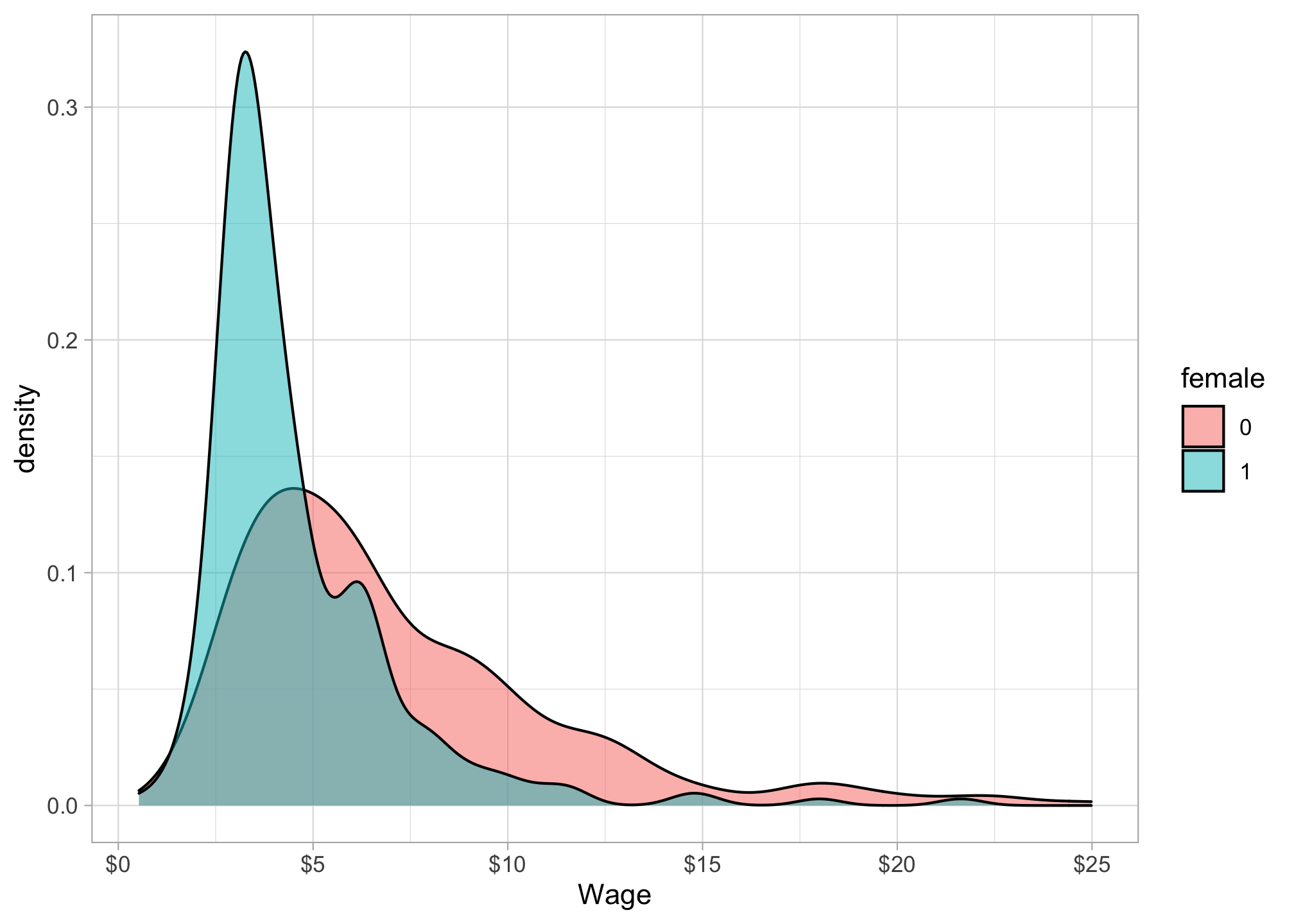

Knowing the distributions of male and female average hourly earnings, we can estimate the sampling distribution of the difference in group eans between men and women as:

The mean: $$\begin{array}{cc}\overline{d}& ={\overline{Y}}_M-{\overline{Y}}_W\\ \overline{d}& =7.10-4.59\\ \overline{d}& =2.51\end{array}$$

The standard error of the mean: $$\begin{array}{cc}SE\left(\overline{d}\right)& =\sqrt{\frac{s_M^2}{n_M}+\frac{s_W^2}{n_W}}\\ & =\sqrt{\frac{{4.16}^2}{274}+\frac{{2.33}^2}{252}}\\ & \approx 0.29\end{array}$$

So the sampling distribution of the difference in group means is distributed: $$\overline{d}\sim N(2.51,0.29)$$

ggplot(data = data.frame(x = 0:6))+
  aes(x = x)+
  stat_function(fun = dnorm, args = list(mean = 2.51, sd = 0.29), color = "purple")+
  labs(x = "Wage Difference",
       y = "Density")+
  scale_x_continuous(breaks = seq(0,6,1),
                     labels = scales::dollar)+
  theme_light()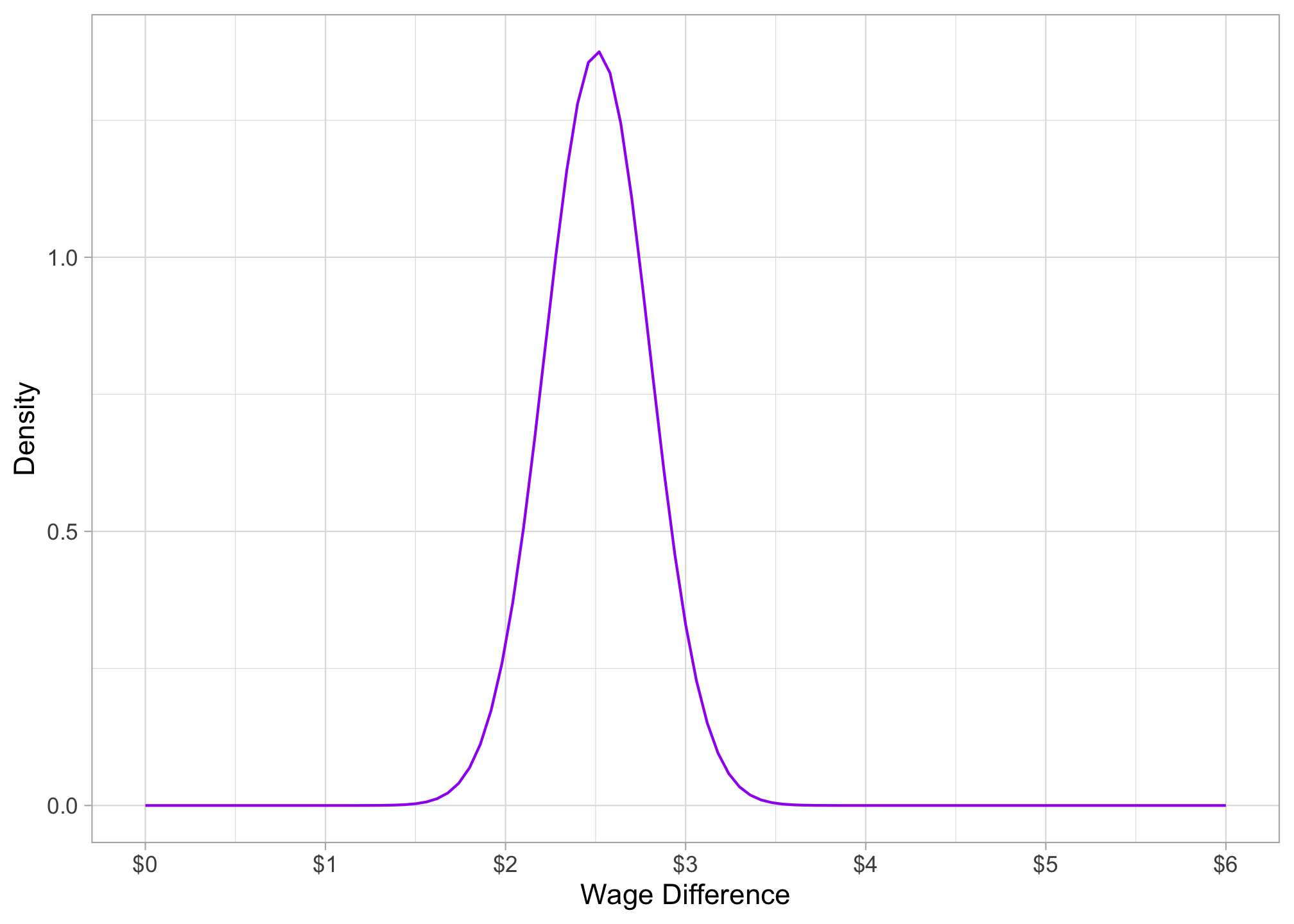

Now we the $t$-test like any other:

$$\begin{array}{cc}t& =\frac{\text{estimate}-\text{null hypothesis}}{\text{standard error of the estimate}}\\ & =\frac{d-0}{SE\left(d\right)}\\ & =\frac{2.51-0}{0.29}\\ & =8.66\end{array}$$

This is statistically significant. The $p$-value, $P(t>8.66)=$ is 0.000000000000000000410, or basically, 0.

pt(8.66,456.33, lower.tail = FALSE)

## [1] 4.102729e-17

The $t$-test in R

t.test(wage ~ female, data = wages, var.equal = FALSE)

## 
##  Welch Two Sample t-test
## 
## data:  wage by female
## t = 8.44, df = 456.33, p-value = 4.243e-16
## alternative hypothesis: true difference in means between group 0 and group 1 is not equal to 0
## 95 percent confidence interval:
##  1.926971 3.096690
## sample estimates:
## mean in group 0 mean in group 1 
##        7.099489        4.587659

reg <- lm(wage~female, data = wages)
summary(reg)

## 
## Call:
## lm(formula = wage ~ female, data = wages)
## 
## Residuals:
##     Min      1Q  Median      3Q     Max 
## -5.5995 -1.8495 -0.9877  1.4260 17.8805 
## 
## Coefficients:
##             Estimate Std. Error t value Pr(>|t|)    
## (Intercept)   7.0995     0.2100  33.806  < 2e-16 ***
## female1      -2.5118     0.3034  -8.279 1.04e-15 ***
## ---
## Signif. codes:  0 '***' 0.001 '**' 0.01 '*' 0.05 '.' 0.1 ' ' 1
## 
## Residual standard error: 3.476 on 524 degrees of freedom
## Multiple R-squared:  0.1157, Adjusted R-squared:  0.114 
## F-statistic: 68.54 on 1 and 524 DF,  p-value: 1.042e-15