Overview
Today we finish your crash course/review of basic statistics with random variables and distributions.
Readings
- Math and Probability Background Appendices B-I in Bailey, Real Econometrics
Now that we return to the statistics, we will do a minimal overview of basic statistics and distributions. Review all of Bailey’s appendices.
Slides
Below, you can find the slides in two formats. Clicking the image will bring you to the html version of the slides in a new tab. Note while in going through the slides, you can type h to see a special list of viewing options, and type o for an outline view of all the slides.
The lower button will allow you to download a PDF version of the slides. I suggest printing the slides beforehand and using them to take additional notes in class (not everything is in the slides)!

R Practice
Answers from last class’ practice problems on base R are posted on that page. Today’s “practice problems” get you to practice the tools we are working with today. They are again not required, but will help you if you are interested.
Assignments
Problem Set 1
Problem Set 1 is posted and is due by class Tuesday September 14. Please see the instructions for more information on how to submit your assignment (there are multiple ways!).
Problem set 2 (on classes 2.1-2.2) will be posted shortly, and will be due by Tuesday September 21.
Math Appendix
Properties of Expected Value and Variance
There are several useful mathematical properties of expected value and variance.
Property 1: the expected value of a constant is itself, and the variance of a constant is 0.
\[\begin{align*} E(c)&=c\\ var(c)&=0\\ sd(c)&=0\\ \end{align*}\]
For any constant, \(c\)
- Example: \(E(2)=2\), \(var(2)=0\), \(sd(2)=0\)
Property 2: adding or subtracting a constant to a random variable and then taking the mean or variance:
\[\begin{align*} E(X \pm c)&=E(X) \pm c\\ var(X \pm c)&=X\\ sd(X \pm c)&=X\\ \end{align*}\]
For any constant, \(c\)
- Example: \(E(2+X)=2+E(X)\), \(var(2+X)=var(X)\), \(sd(2+X)=sd(X)\)
Property 3: multiplying a constant to a random variable and then taking the mean or variance:
\[\begin{align*} E(aX)&=E(X) aE(X)\\ var(aX)&=a^2var(X)\\ sd(aX)&=|a|sd(X)\\ \end{align*}\]
For any constant, \(a\)
- Example: \(E(2X)=2E(X)\), \(var(2X)=4var(X)\), \(sd(2X)=2sd(X)\)
Property 4: the expected value of the sum of two random variables is equal to the sum of each random variable’s expected value:
\[E(X \pm Y)=E(X) \pm E(Y)\]
R Appendix
Creating Mathematical Functions
You can create custom mathematical functions using mosaic by defining an R function() with multiple arguments. As a simple example, make the function \(f(x) = 10x-x^2\) (with one argument, \(x\) since it is a univariate function) as follows:
# store as a named function, I'll call it "my_function"
my_function<-function(x){10*x-x^2}

# look at it
my_function
## function(x){10*x-x^2}There are some notational requirements from R for making functions. Any coefficient in front of a variable (such as the 10 in 10x must be explicitly multiplied by the variable, as in 10*x).
To use the function to calculate its value at a particular value of x, simply define what the (x) is and run your named function on it:
# f of 2
my_function(2)
## [1] 16# f of 2 and 4
my_function(c(2,4))## [1] 16 24# f of 2 through 7
my_function(2:7)## [1] 16 21 24 25 24 21# ALTERNATIVELY
# define x first as a vector and then run function on it
x<-c(2,4)
my_function(x)## [1] 16 24Graphing Mathematical Functions
In ggplot there is a dedicated stat_function() (equivalent to a geom_ layer) to graph mathematical and statistical functions. All that is needed is a data.frame of a range of x values to act as the source for data, and set x equal to those values for aesthetics.
library(tidyverse)## ── Attaching packages ─────────────────────────────────────── tidyverse 1.3.1 ──## ✓ ggplot2 3.3.5 ✓ purrr 0.3.4
## ✓ tibble 3.1.4 ✓ dplyr 1.0.7
## ✓ tidyr 1.1.3 ✓ stringr 1.4.0
## ✓ readr 2.0.0 ✓ forcats 0.5.1## ── Conflicts ────────────────────────────────────────── tidyverse_conflicts() ──
## x dplyr::filter() masks stats::filter()
## x dplyr::lag() masks stats::lag()# x values are integers 1 through 10
ggplot(data = data.frame(x = 1:10))+
aes(x = x)
Then we add the stat_function, where fun = is the most important argument where you define the to function to graph as your function created above, for example, our my_function.
ggplot(data = data.frame(x = 1:10))+
  aes(x = x)+
stat_function(fun = my_function) 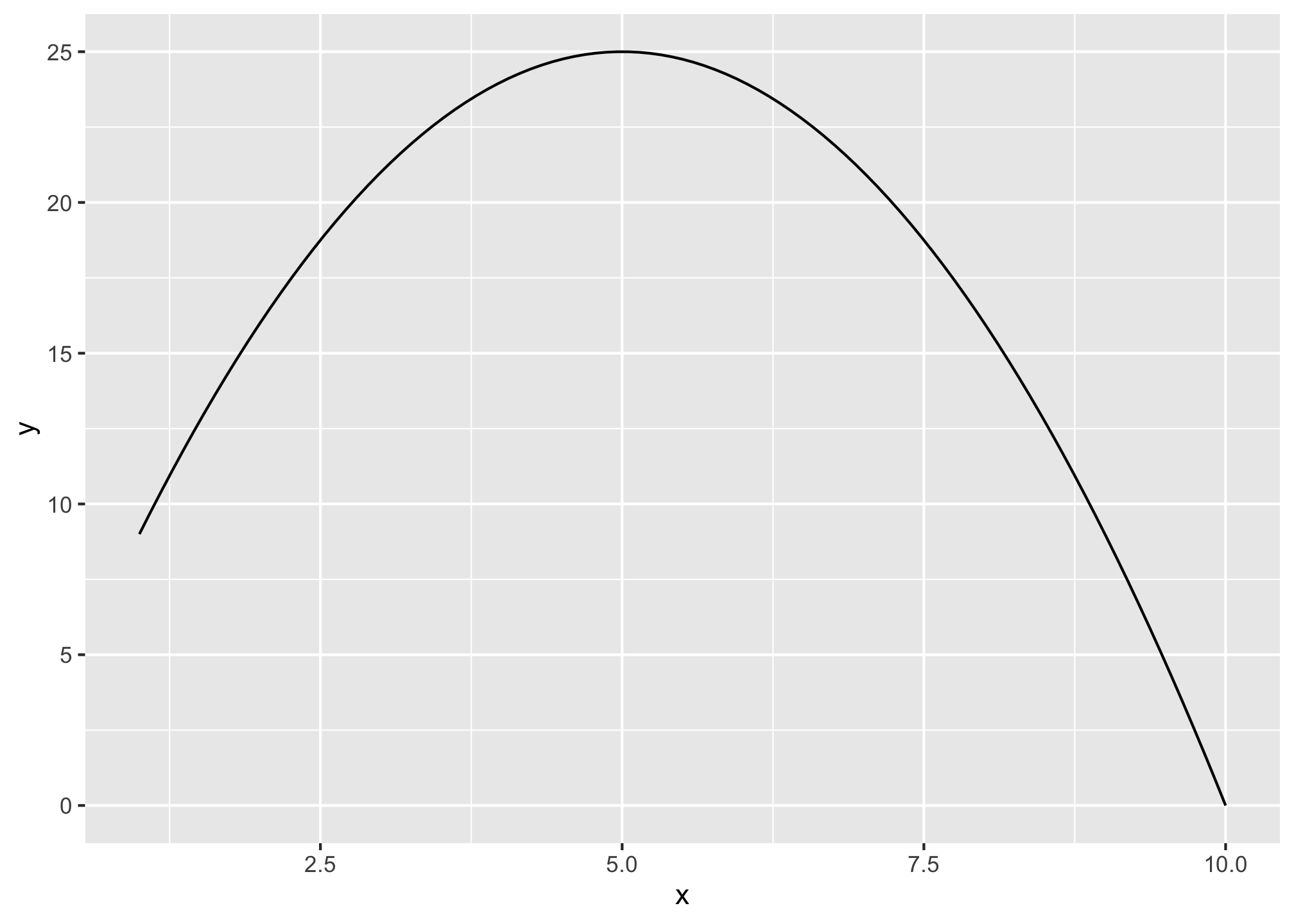
You can also adjust things like size, color, and line type.
ggplot(data = data.frame(x = 1:10))+
  aes(x = x)+
stat_function(fun = my_function, color = "blue", size = 2, linetype = "dashed") 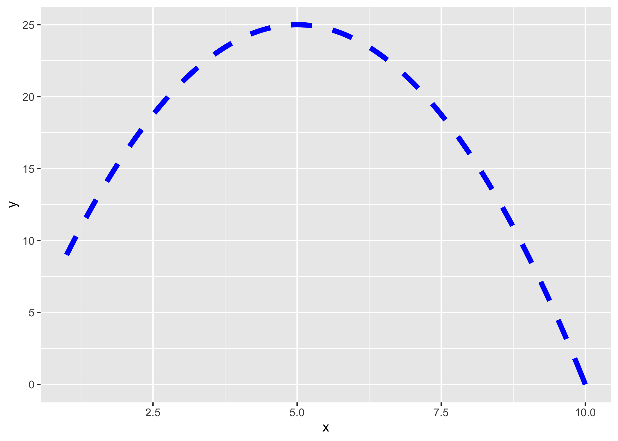
Bult-in Statistical Functions
There are some standard statistical distributions built into R. They require a combination of a specific prefix and a distribution.
Prefixes:
| Action/Type | Prefix |
|---|---|
| random draw | r |
| density (pdf) | d |
| cumulative density (cdf) | p |
| quantile (inverse cdf) | q |
Distributions:
| Distribution | Name in R |
|---|---|
| Normal | norm |
| Uniform | unif |
| Student’s t | t |
| Binomial | binom |
| Negative binomial | nbinom |
| Hypergeometric | hyper |
| Weibull | weibull |
| Beta | beta |
| Gamma | gamma |
Thus, what you want is a combination of the prefix and the distribution.
Some common examples:
- Take random draws from a normal distribution:
rnorm(n = 10, # take 10 draws from a normal distribution with:
      mean = 2, # mean of 2
      sd = 1) # sd of 1
## [1] 0.9306446 1.9587986 1.7016603 1.2481484 1.3399839 1.9677189 0.3313595
## [8] 1.6183993 2.5601664 0.5277235- Get probability of a random variable being less than or equal to a value (cdf) from a normal distribution:
# find probability of area to the LEFT of a number on pdf (note this = cdf of that number!)
pnorm(q = 80, # number is 80 from a distribution where:
      mean = 200, # mean is 100
      sd = 100, # sd is 100
      lower.tail = TRUE) # looking to the LEFT in lower tail
## [1] 0.1150697- Find the value of a distribution that is a specified percentile.
# find the 38th percentile value
qnorm(p = 0.38, # 38th percentile from a distribution where:
      mean = 200, # mean is 200
      sd = 100) # sd is 100
## [1] 169.4519Graphing Statistical Functions
You can also graph these commonly used statistical functions by setting fun = the named functions in your stat_function() layer. If you want to specify the mean and standard deviation, use args = list() to include the required arguments from the named function above (e.g. dnorm needs mean and sd).
ggplot(data = data.frame(x = -400:600))+
  aes(x = x)+
stat_function(fun = dnorm, args = list(mean = 200, sd = 200), color = "blue", size = 2, linetype = "dashed") 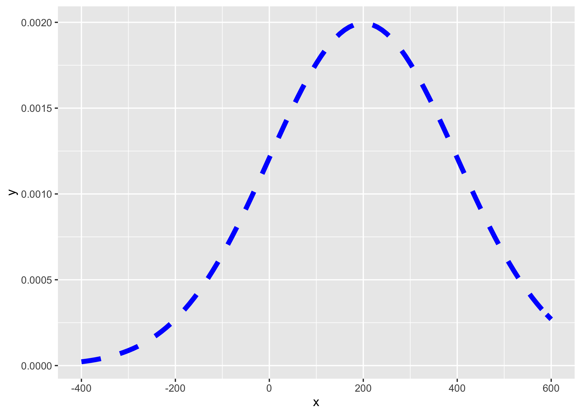
If you don’t include this, it will graph the standard distribution:
ggplot(data = data.frame(x = -4:4))+
  aes(x = x)+
stat_function(fun = dnorm, color = "blue", size = 2, linetype = "dashed") 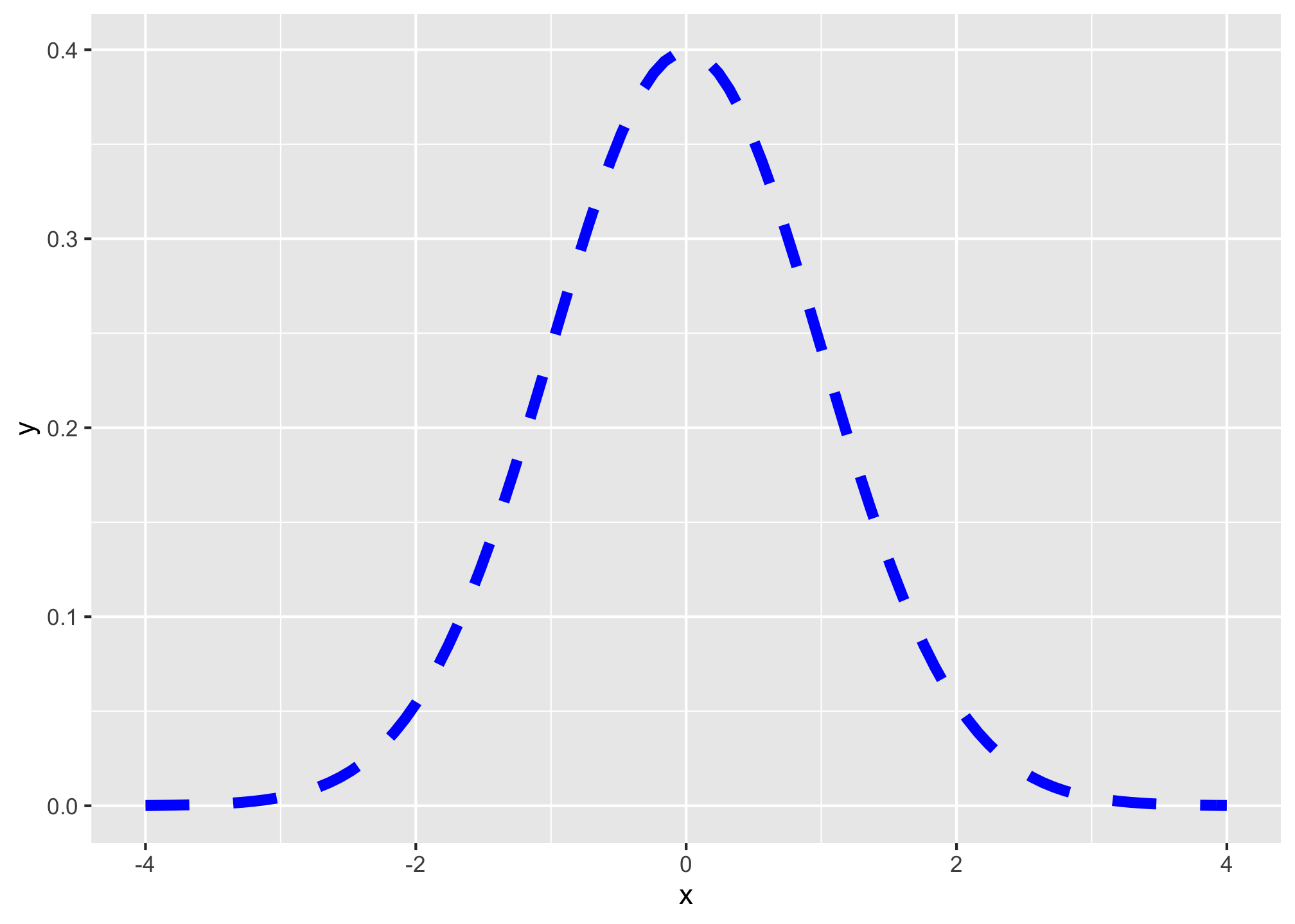
To add shading under a distribution, simply add a duplicate of the stat_function() layer, but add geom="area" to indicate the area beneath the function should be filled, and you can limit the domain of the fill with xlim=c(start,end), where start and end are the x-values for the endpoints of the fill.
# graph normal distribution and shade area between -2 and 2
ggplot(data = data.frame(x = -4:4))+
  aes(x = x)+
  stat_function(fun = dnorm, color = "blue", size = 2, linetype = "dashed")+
  stat_function(fun = dnorm, xlim = c(-2,2), geom = "area", fill = "green", alpha=0.5)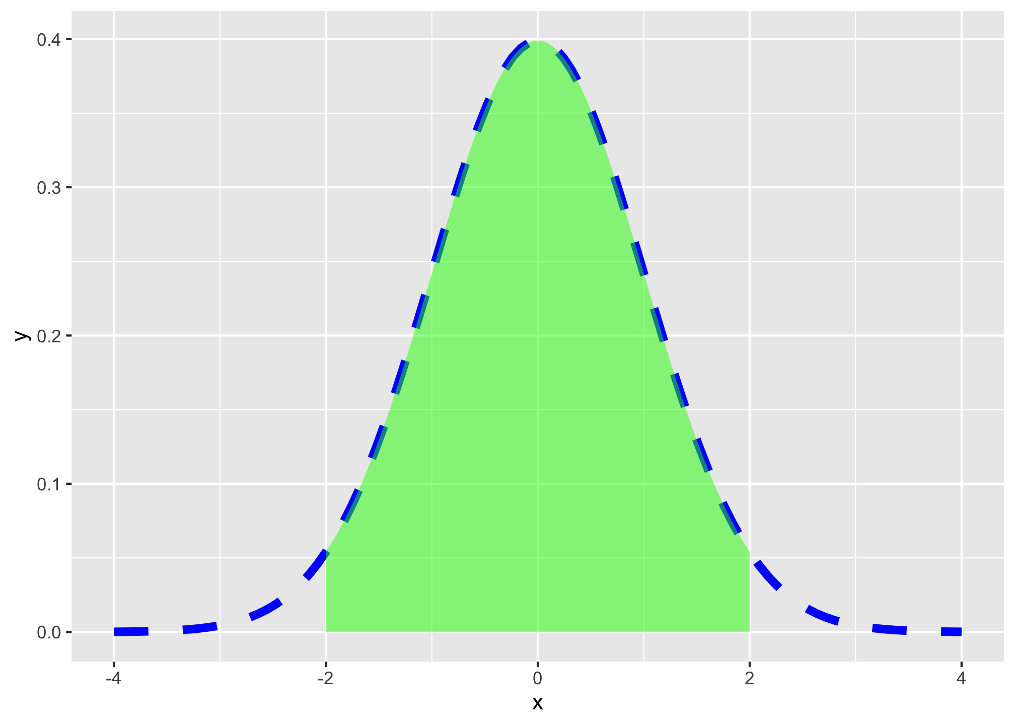
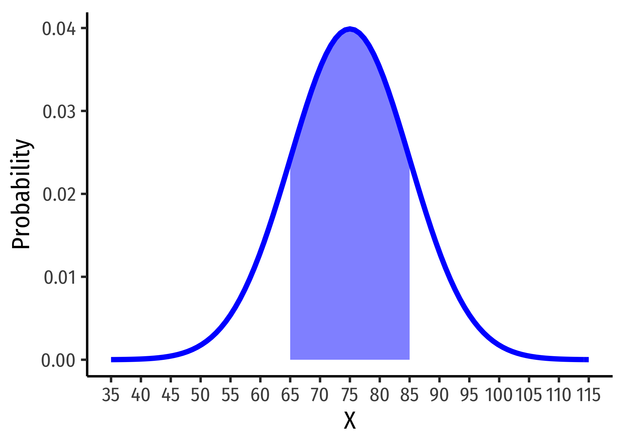
Hence, here is one graph from my slides:
ggplot(data = tibble(x=35:115))+
  aes(x = x)+
  stat_function(fun = dnorm, args = list(mean = 75, sd = 10), size = 2, color="blue")+
  stat_function(fun = dnorm, args = list(mean = 75, sd = 10), geom = "area", xlim = c(65,85), fill="blue", alpha=0.5)+
  labs(x = "X",
       y = "Probability")+
  scale_x_continuous(breaks = seq(35,115,5))+
  theme_classic(base_family = "Fira Sans Condensed",
           base_size=20)