2.3 — OLS Linear Regression — Class Content

Problem Set 1

Problem Set 2 is due by Tuesday September 21. Please see the instructions for more information on how to submit your assignment (there are multiple ways!).

Variance

Recall the variance of a discrete random variable \(X\), denoted \(var(X)\) or \(\sigma^2\), is the expected value (probability-weighted average) of the squared deviations of \(X_i\) from it’s mean (or expected value) \(\bar{X}\) or \(E(X)\).²

\[\begin{align*} \sigma_X^2&=E(X-E(X))\\ &=\sum^n_{i=1} (X_i-\bar{X})^2 p_i \end{align*}\]

Fpr continuous data (if all possible values of \(X_i\) are equally likely or we don’t know the probabilities), we can write variance as a simple average of squared deviations from the mean:

\[\begin{align*} \sigma_X^2&=\frac{1}{n}\sum^n_{i=1}(X_i-\bar{X})^2 \end{align*}\]

Variance has some useful properties:

Property 1: The variance of a constant is 0

\[var(c)=0 \text{ iff } P(X=c)=1\]

If a random variable takes the same value (e.g. 2) with probability 1.00, \(E(2)=2\), so the average squared deviation from the mean is 0, because there are never any values other than 2.

Property 2: The variance is unchanged for a random variable plus/minus a constant

\[var(X\pm c)\]

Since the variance of a constant is 0.

Property 3: The variance of a scaled random variable is scaled by the square of the coefficient

\[var(aX)=a^2var(X)\]

Property 4: The variance of a linear transformation of a random variable is scaled by the square of the coefficient

\[var(aX+b)=a^2var(X)\]

Covariance

For two random variables, \(X\) and \(Y\), we can measure their covariance (denoted \(cov(X,Y)\) or \(\sigma_{X,Y}\))³ to quantify how they vary together. A good way to think about this is: when \(X\) is above its mean, would we expect \(Y\) to also be above its mean (and covary positively), or below its mean (and covary negatively). Remember, this is describing the joint probability distribution for two random variables.

\[\begin{align*} \sigma_{X,Y}&=E\big[(X-\bar{X})(Y-\bar{Y})\big] \end{align*}\]

Again, in the case of equally probable values for both \(X\) and \(Y\), covariance is sometimes written:

\[\begin{align*} \sigma_{X,Y}&=\frac{1}{N}\sum_{i=1}^n(X-\bar{X})(Y-\bar{Y}) \end{align*}\]

Covariance also has a number of useful properties:

Property 1: The covariance of a random variable \(X\) and a constant \(c\) is 0

\[cov(X,c)=0\]

Property 2: The covariance of a random variable and itself is the variable’s variance

\[\begin{align*} cov(X,X)&=var(X)\\ \sigma_{X,X}&=\sigma^2_X\\ \end{align*}\]

Property 3: The covariance of a two random variables \(X\) and \(Y\) each scaled by a constant \(a\) and \(b\) is the product of the covariance and the constants

\[cov(aX,bY)=a\times b \times cov(X,Y)\]

Property 4: If two random variables are independent, their covariance is 0

\[cov(X,Y)=0 \text{ iff } X \text{ and } Y \text{ are independent:} E(XY)=E(X)\times E(Y)\]

Correlation

Covariance, like variance, is often cumbersome, and the numerical value of the covariance of two random variables does not really mean much. It is often convenient to normalize the covariance to a decimal between \(-1\) and 1. We do this by dividing by the product of the standard deviations of \(X\) and \(Y\). This is known as the correlation coefficient between \(X\) and \(Y\), denoted \(corr(X,Y)\) or \(\rho_{X,Y}\) (for populations) or \(r_{X,Y}\) (for samples):

\[\begin{align*} r_{X,Y}&=\frac{cov(X,Y)}{sd(X)sd(Y)}\\ &=\frac{E\big[(X-\bar{X})(Y-\bar{Y})\big]}{\sqrt{E\big[X-\bar{X}\big]}\sqrt{E\big[Y-\bar{Y}\big]}}\\ &=\frac{\sigma_{X,Y}}{\sigma_X \sigma_Y}\\ \end{align*}\]

Note this also means that covariance is the product of the standard deviation of \(X\) and \(Y\) and their correlation coefficient:

\[\begin{align*} \sigma_{X,Y}&=r_{X,Y}\sigma_X \sigma_Y \\ cov(X,Y)&=corr(X,Y)\times sd(X) \times sd(Y) \\ \end{align*}\]

Another way to reach the (sample) correlation coefficient is by finding the average joint \(Z\)-score of each pair of \((X_i,Y_i)\):

\[\begin{align*} r_{X,Y}&=\frac{1}{n}\frac{\displaystyle\sum^n_{i=1}(X_i-\bar{X})(Y_i-\bar{Y}))}{s_X s_Y} && \text{Definition of sample correlation}\\ &=\frac{1}{n}\displaystyle\sum^n_{i=1}\bigg(\frac{X_i-\bar{X}}{s_X}\bigg)\bigg(\frac{Y_i-\bar{Y}}{s_Y}\bigg) && \text{Breaking into separate sums} \\ &=\frac{1}{n}\displaystyle\sum^n_{i=1}(Z_X)(Z_Y) && \text{Recognize each sum is the z-score for that r.v.} \\ \end{align*}\]

Correlation has some useful properties that should be familiar to you:

• Correlation is between \(-1\) and 1
• A correlation of -1 is a downward sloping straight line
• A correlation of 1 is an upward sloping straight line
• A correlation of 0 implies no relationship

library(tidyverse)

corr_example<-tibble(x=c(1,2,3,4),
                         y=c(1,2,4,9))

ggplot(corr_example,aes(x=x,y=y))+geom_point()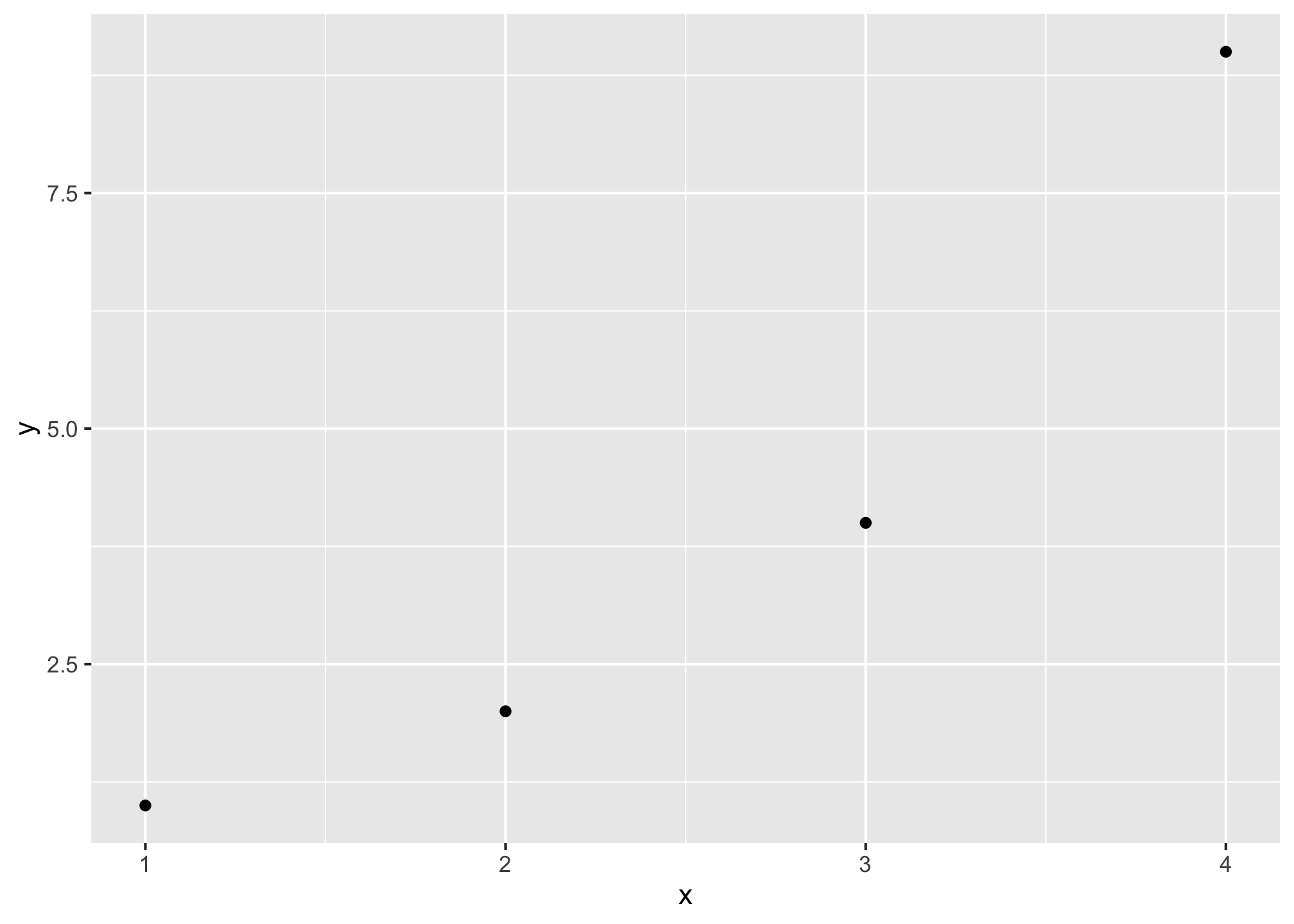

corr_example %>%
  summarize(mean_x = mean(x), #find mean of x, its 2.5
            sd_x = sd(x), #find sd of x, its 1.291
            mean_y = mean(y), #find mean of y, its 4
            sd_y = sd(y)) #find sd of y, its 3.559

## # A tibble: 1 × 4
##   mean_x  sd_x mean_y  sd_y
##    <dbl> <dbl>  <dbl> <dbl>
## 1    2.5  1.29      4  3.56

#take z score of x,y for each pair and multiply them

corr_example <- corr_example %>%
  mutate(z_product = ((x-mean(x))/sd(x)) * ((y-mean(y))/sd(y)))

corr_example %>%
  summarize(avg_z_product = sum(z_product)/(n()-1), # average z products over n-1
            actual_corr = cor(x,y), #compare our answer to actual cor() command!
            covariance = cov(x,y)) # just for kicks, what's the covariance? 

## # A tibble: 1 × 3
##   avg_z_product actual_corr covariance
##           <dbl>       <dbl>      <dbl>
## 1         0.943       0.943       4.33