Overview
Today we begin extending the foundation of simple linear regression with one variable into more advanced models that can plausibly claim (when we are done) to measure causal relationships between and . The rest of the semester is primarily extending regression from one to many, and changing the functional form to fit various idiosyncracies of different variables, or use clever techniques to isolate marginal effects of interest.
We begin by covering the fundamental problem of causal inference, that we can never observe counterfactual states of the world. If we could, then we could easily measure the causal effect of by comparing how is different when is different. The next best thing we can do is run a random control trial (RCT) where individuals are randomly assigned to groups to be given (different) treatment(s), and then we can compare the average outcome across groups. Random assignment ensures the only thing that differs across group outcomes is whether or not the group was given treatment, estimating the causal effect of treatment on the outcome.
For now, we will understand causality to mean the average treatment effect (ATE) from a RCT. RCTs are both popular and controversial. Last year’s Nobel Prize winners in economics won for their use of RCTs in development economics, but they have drawn significant criticism from other top economists as not being sufficiently generalizable.
Of course, the bigger problem is it is very difficult, often impossible, to run a RCT to test a hypothesis. So economists have developed a toolkit of clever techniques to identify causal effects in “natural experiments” or “quasi-experiments” that sufficiently simulate a RCT. Knowledge of this repertoire of tools is truly why modern economists are in demand by government and business (not supply and demand models, etc)!
Readings
- Ch.1 in Bailey, Real Econometrics
- Ch. 4 in Cunningham (2020), Causal Inference, the Mixtape
- Rubin Causal Model
Bailey begins the book with a discussion of causality and random control trials that is pretty good.
The potential outcomes notation (e.g. and and model comes from a very famous 1974 paper by Donald Rubin in psychology. You can read more about it in Cunningham (2020) above, or the Wikipedia entry on the model.
Scott Cunningham’s excellent (and free!) Causal Inference, the Mixtape has a great discussion of the history, and examples, of potential outcomes in an accessible way.
The classic example that most economists (including myself) were taught about causality is the treatment of the Rubin model in Angrist and Pischke’s Mostly Harmless Econometrics (one of the classic books on econometrics). You do not need to buy that book for this class, but if you will be doing data work in your future, or going to graduate school, this book is a must own and read:
My health insurance example is lifted directly out of this book.
Here’s also a great list of famous social science (including economics) papers that use natural experiments:
For more on John Snow and the birth of epidemiology, the excellent PBS show Victoria has a full episode (and great resources) about the cholera outbreak.
Slides
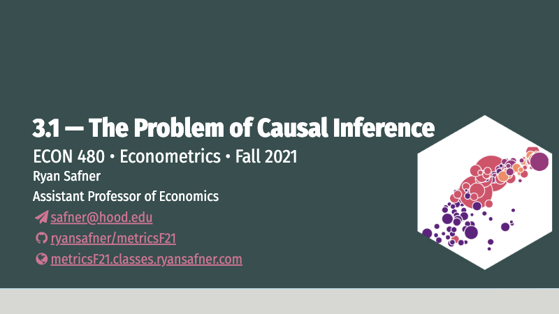
Below, you can find the slides in two formats. Clicking the image will bring you to the html version of the slides in a new tab. Note while in going through the slides, you can type h to see a special list of viewing options, and type o for an outline view of all the slides.
The lower button will allow you to download a PDF version of the slides. I suggest printing the slides beforehand and using them to take additional notes in class (not everything is in the slides)!
