Overview
Today we continue examining how to use categorical data in regression, particularly focusing on interactions between variables. We look at three types of interaction effects: 1. Interaction between a continuous variable & a dummy variable 2. Interaction between two dummy variables 3. Interaction between two continuous variables
We will also be working on practice problems today in R.
Slides
Below, you can find the slides in two formats. Clicking the image will bring you to the html version of the slides in a new tab. Note while in going through the slides, you can type h to see a special list of viewing options, and type o for an outline view of all the slides.
The lower button will allow you to download a PDF version of the slides. I suggest printing the slides beforehand and using them to take additional notes in class (not everything is in the slides)!

R Practice
Today you will be working on R practice problems on multivariate regression. Answers will be posted later on that page.
Assignments
Problem Set 4 Due Tues Nov 9
Problem Set 4 is due by the end of the day on Tuesday, November 9.
Appendix: Marginal Effects for Two-Continuous Variable Interactions
In class, we looked at the effects of education on wages, experience on wages, and the interaction between education and experience on wages:
Using the wage1 data in the wooldridge package, we found the following:
library(tidyverse)
library(broom)
library(wooldridge)
wages <- wage1
reg_cont <- lm(wage ~ educ + exper + educ:exper, data = wages)
reg_cont %>% tidy()
## # A tibble: 4 × 5
## term estimate std.error statistic p.value
## <chr> <dbl> <dbl> <dbl> <dbl>
## 1 (Intercept) -2.86 1.18 -2.42 1.58e- 2
## 2 educ 0.602 0.0899 6.69 5.64e-11
## 3 exper 0.0458 0.0426 1.07 2.83e- 1
## 4 educ:exper 0.00206 0.00349 0.591 5.55e- 1Let’s extract and save each of these ’s for later use.
b_1 <- reg_cont %>%
  tidy() %>%
  filter(term == "educ") %>%
  pull(estimate)

b_2 <- reg_cont %>%
  tidy() %>%
  filter(term == "exper") %>%
  pull(estimate)

b_3 <- reg_cont %>%
  tidy() %>%
  filter(term == "educ:exper") %>%
  pull(estimate)

# let's check each of these
b_1
## [1] 0.6017355b_2## [1] 0.04576891b_3## [1] 0.002062345We know that the marginal effect of each of the two variables on depends on the value of the other variable:
| Variable | Marginal Effect on Wages (Formula) | Marginal Effect on Wages (Estimate) |
|---|---|---|
| Education | 0.6017355 + 0.0020623 | |
| Experience | 0.6017355 + 0.0020623 |
We can get the marginal effects more precisely by making a function of each marginal effect, using the coefficients saved above. To make a your own function in R (a very handy thing to do!), simply define an object as my_function<- function(){}. Inside the () goes any arguments the function will need (here, it’s the value of the other variable), and then the formula to apply to that argument. Then you can run the function on any object.
As a simple example, to make a function that squares x:
# make function called "square" that squares x
square<-function(x){x^2}

# test it on the value 4
square(4)## [1] 16# test it on all of these values
square(1:4)## [1] 1 4 9 16Now let’s make a function for the marginal effect of education (by experience):
# make marginal effect of education on wages by years of experience function
# input is years of experience
me_educ<-function(exper){b_1*b_3*exper}

# now its a function, let's input 5 years, 10 years, 15 years of experience
me_educ(c(5,10,15))
## [1] 0.006204929 0.012409858 0.018614788Now let’s make a function for the marginal effect of experience (by education):
# make marginal effect of experience on wages by years of education function
# input is years of education
me_exper<-function(educ){b_2*b_3*educ}

# now its a function, let's input 5 years, 10 years, 15 years of education
me_exper(c(5,10,15))
## [1] 0.0004719563 0.0009439126 0.0014158689We can now graph these
margin_educ<-ggplot(data = wages)+
  aes(x = exper)+
  stat_function(fun = me_educ, geom = "line", color = "blue")+
  scale_y_continuous(labels = scales::dollar)+
  labs(x = "Years of Experience",
       y = "Marginal Effect of Education on Wages",
       title = "Effect of Education on Wages, by Years of Experience")+
  ggthemes::theme_pander(base_family = "Fira Sans Condensed", base_size = 14)
margin_educ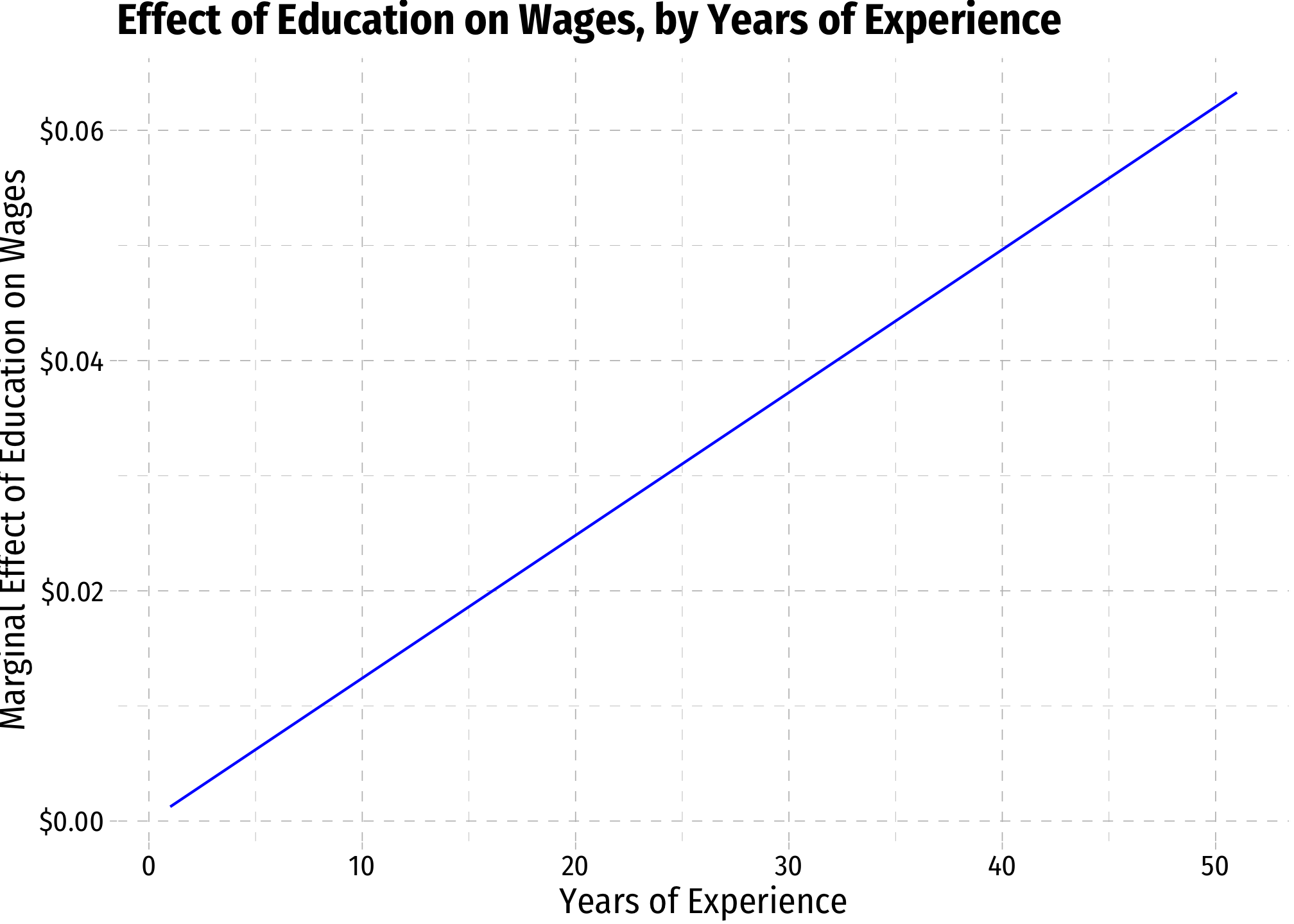
margin_exper<-ggplot(data = wages)+
  aes(x = educ)+
  stat_function(fun = me_exper, geom = "line", color = "blue")+
  scale_y_continuous(labels = function(x){paste0("$",x)})+
  labs(x = "Years of Education",
       y = "Marginal Effect of Experience on Wages",
       title = "Effect of Experience on Wages, by Years of Education")+
  ggthemes::theme_pander(base_family = "Fira Sans Condensed", base_size = 14)
margin_exper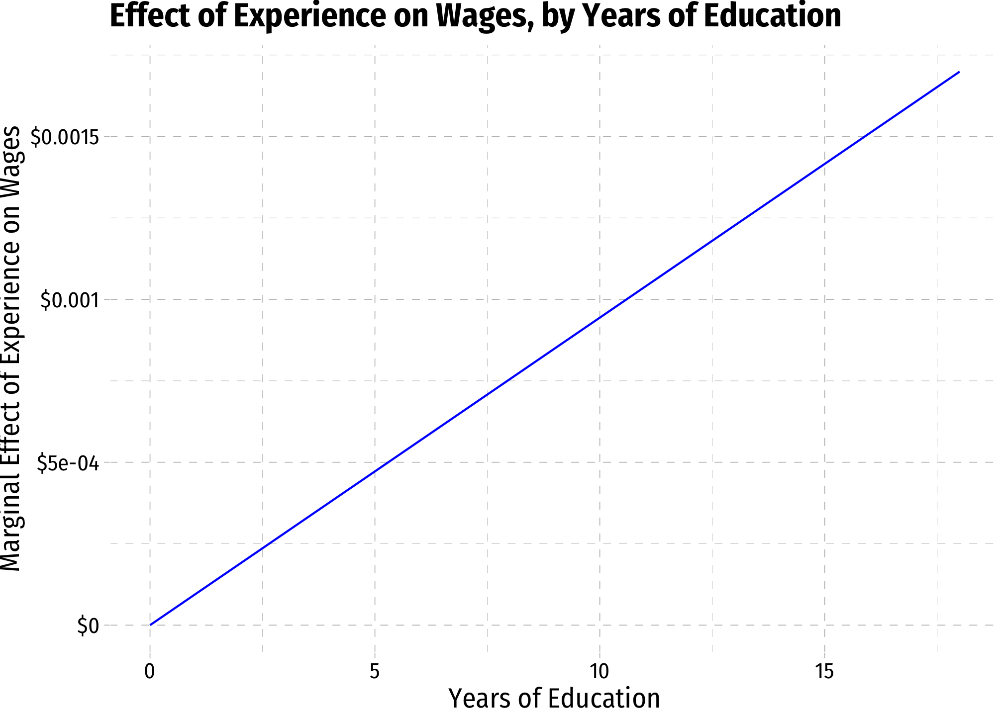
Standard Error of Marginal Effects
If we want to add the standard error to these graphs, we need to extract the ’s from the original regression output:
se_b_1 <- reg_cont %>%
  tidy() %>%
  filter(term == "educ") %>%
  pull(std.error)

se_b_2 <- reg_cont %>%
  tidy() %>%
  filter(term == "exper") %>%
  pull(std.error)

se_b_3 <- reg_cont %>%
  tidy() %>%
  filter(term == "educ:exper") %>%
  pull(std.error)

# let's check each of these
se_b_1
## [1] 0.08989998se_b_2## [1] 0.04261376se_b_3## [1] 0.003490614Now the standard error of the marginal effect is a bit tricky. The marginal effect, for example, of Education on Wages, we saw was . One property of variances (or, when square rooted, standard errors) of random variables is that:
Here, the ’s are random variables, and is a constant (some number, like . So the variance is:
The standard error then is the square root of this. To get the covariance of and , we need to extract it from something called the variance-covariance matrix. A regression creates and stores a matrix that contains the covariances of all ’s with each other (and the covariance of any with itself is the variance of that :
# look at variance-covariance matrix
vcov(reg_cont)
## (Intercept) educ exper educ:exper
## (Intercept) 1.394949133 -0.1040894353 -0.0412570602 3.134939e-03
## educ -0.104089435 0.0080820059 0.0031414567 -2.513073e-04
## exper -0.041257060 0.0031414567 0.0018159324 -1.437215e-04
## educ:exper 0.003134939 -0.0002513073 -0.0001437215 1.218438e-05# make it a tibble to work with using tidyverse methods
v<-as_tibble(vcov(reg_cont))
# we want the covariance between beta 1 and beta 3, save as "cov_b1_b3"
cov_b1_b3<-v %>%
slice(2) %>%
pull(`educ:exper`)
cov_b1_b3 # look at it## [1] -0.0002513073# lets also get the covariance between beta 2 and beta 3 (for later)
cov_b2_b3<-v %>%
slice(3) %>%
pull(`educ:exper`)
cov_b2_b3## [1] -0.0001437215# make a function of the variance of the marginal effect of education on wages
var_me_educ=function(experience){(se_b_1)^2+(se_b_3)^2*experience+2*experience*cov_b1_b3}
# now square root it to get standard error
se_me_educ=function(experience){sqrt(var_me_educ(experience))}
# to plot a 95% confidence interval of the marginal effect, lets make upper and lower CI values as a function of experience
CI_me_educ_upper=function(experience){me_educ(experience)+1.96*se_me_educ(experience)}
CI_me_educ_lower=function(experience){me_educ(experience)-1.96*se_me_educ(experience)}
# lets now add these into the data
wages2<-wages %>%
select(exper) %>%
mutate(me_educ = me_educ(exper),
CI_educ_lower = CI_me_educ_lower(exper),
CI_educ_upper = CI_me_educ_upper(exper)
)## Warning in sqrt(var_me_educ(experience)): NaNs produced
## Warning in sqrt(var_me_educ(experience)): NaNs produced# and graph it!
margin_educ+
geom_ribbon(data = wages2, aes(ymin=CI_educ_lower, ymax=CI_educ_upper), fill = "grey70", alpha = 0.5)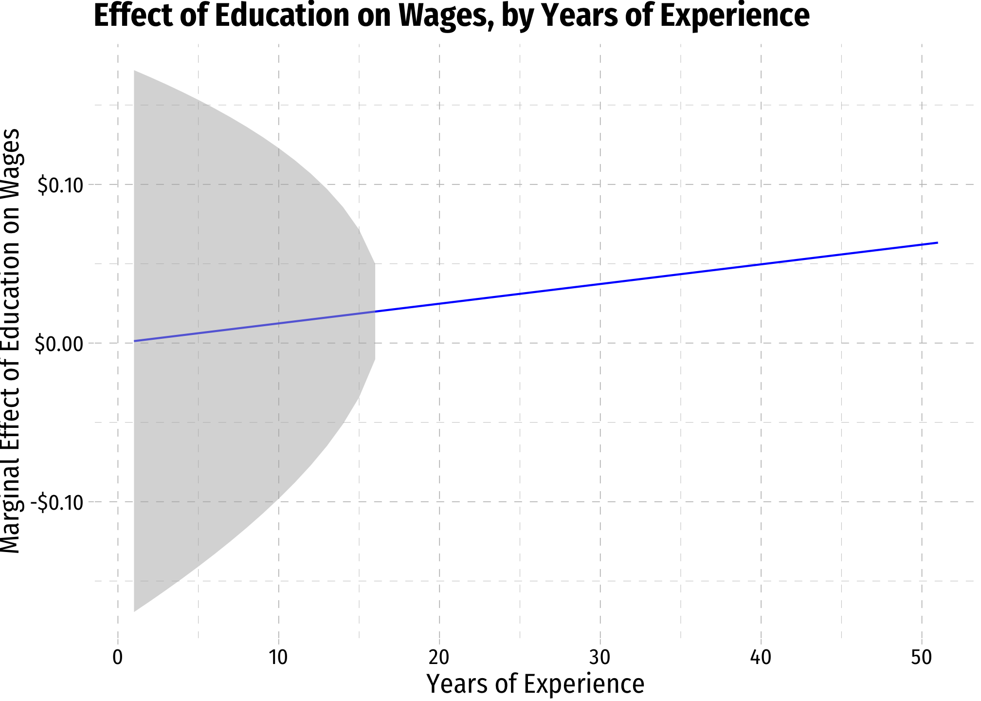
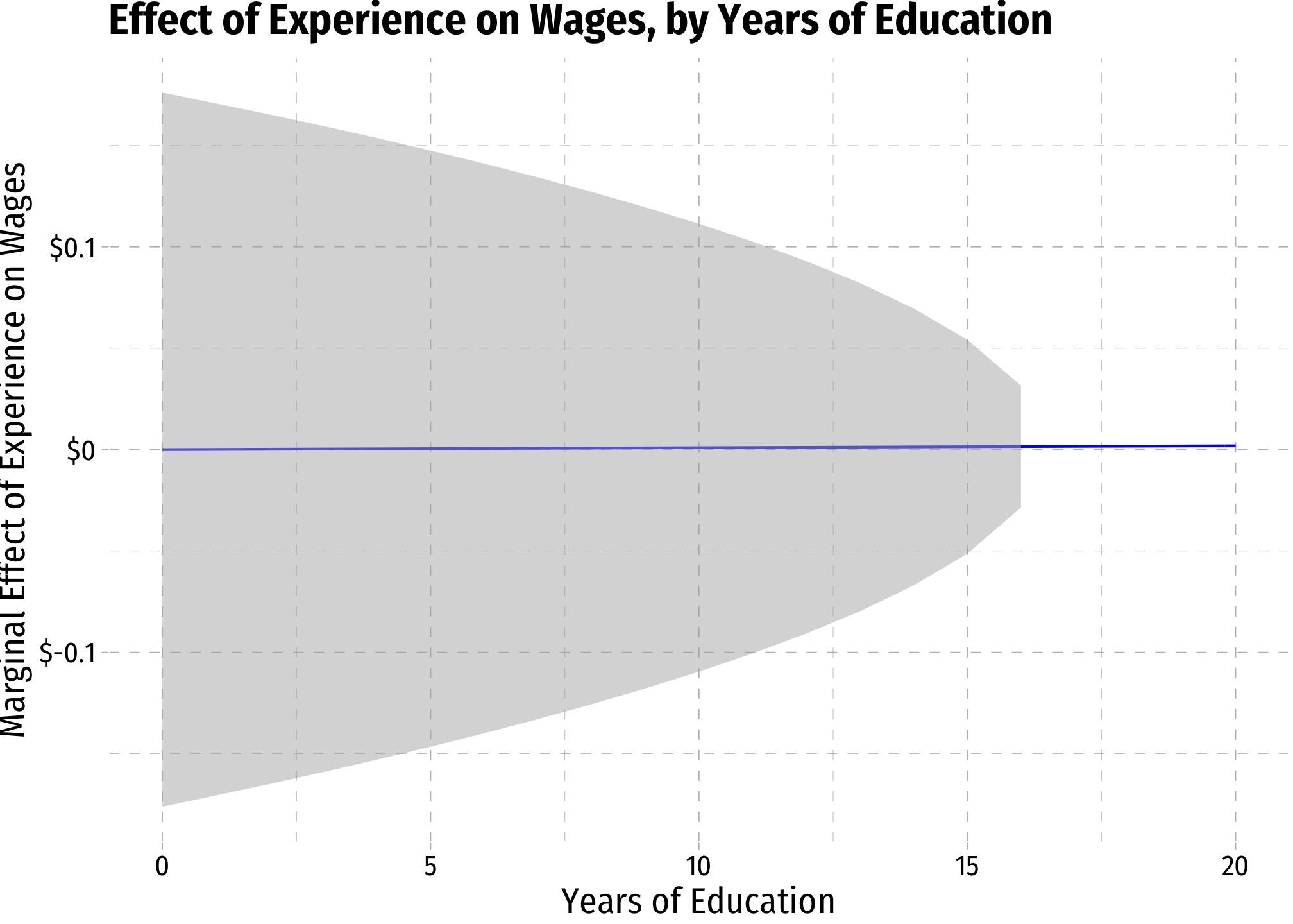
# do the same for the marginal effect of experience on wages
var_me_exper=function(education){(se_b_2)^2+(se_b_3)^2*education+2*education*cov_b2_b3}

# now square root it to get standard error
se_me_exper=function(education){sqrt(var_me_educ(education))}

# to plot a 95% confidence interval of the marginal effect, lets make upper and lower CI values as a function of experience
CI_me_exper_upper=function(education){me_exper(education)+1.96*se_me_exper(education)}
CI_me_exper_lower=function(education){me_exper(education)-1.96*se_me_exper(education)}

# lets now add these into the data
wages3<-wages %>%
  select(educ) %>%
  mutate(me_exper = me_exper(educ),
         CI_exper_lower = CI_me_exper_lower(educ),
         CI_exper_upper = CI_me_exper_upper(educ)
)## Warning in sqrt(var_me_educ(education)): NaNs produced
## Warning in sqrt(var_me_educ(education)): NaNs produced# and graph it!
margin_exper+
geom_ribbon(data = wages3, aes(ymin=CI_exper_lower, ymax=CI_exper_upper), fill = "grey70", alpha = 0.5)+
scale_x_continuous(limits=c(0,20))