3.9 — Logarithmic Regression — Class Content

Overview

Today, we finish up our view of nonlinear models with logarithmic models, which are more frequently used. We also discuss a few other tests and transformations to wrap up multivariate regression before we turn to panel data: standardizing variables to compare effect sizes, and joint hypothesis tests.

Interpretting logged variables can often be difficult to remember, so here I reproduce the tables that describe the interpretations of the marginal effect of $X\to Y$, as well as some visual examples from the slides:

• Hint: the variable that gets logged changes in percent terms, the variable not logged changes in unit terms

Linear-Log	Log-Linear	Log-Log
$\widehat{Y_i}=\widehat{{\beta }_0}+\widehat{{\beta }_1}ln\left(X_i\right)$	$ln\left(\widehat{Y_i}\right)=\widehat{{\beta }_0}+\widehat{{\beta }_1}{X}_i$	$ln\left(\widehat{Y_i}\right)=\widehat{{\beta }_0}+\widehat{{\beta }_1}ln\left(X_i\right)$
$R^2=0.65$	$R^2=0.30$	$R^2=0.61$

Readings

• Ch. 7.1 in Bailey, Real Econometrics

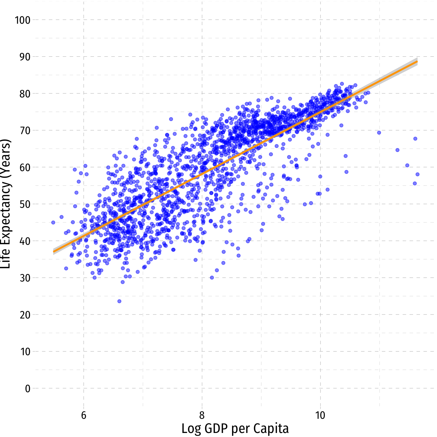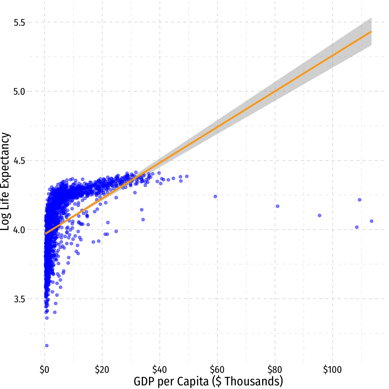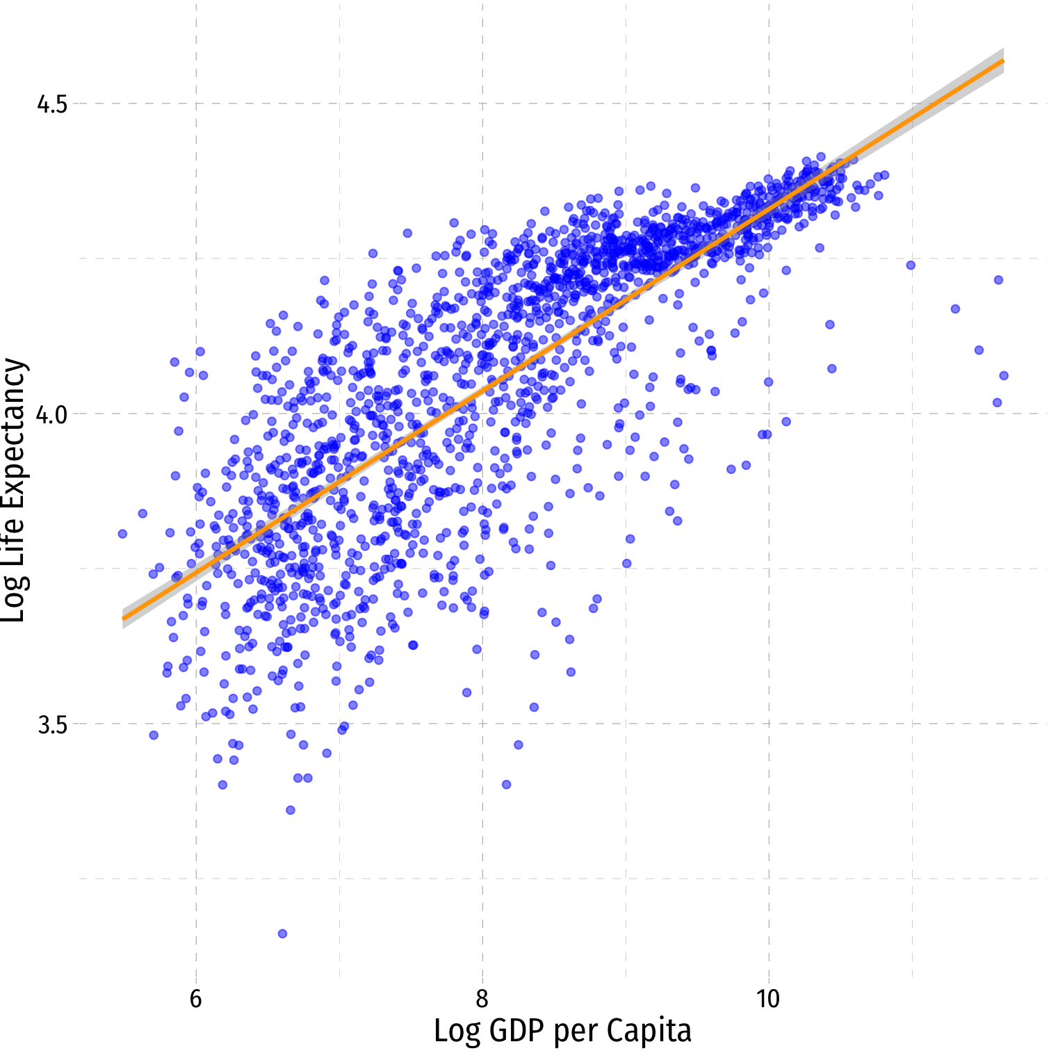Slides

Below, you can find the slides in two formats. Clicking the image will bring you to the html version of the slides in a new tab. Note while in going through the slides, you can type h to see a special list of viewing options, and type o for an outline view of all the slides.

The lower button will allow you to download a PDF version of the slides. I suggest printing the slides beforehand and using them to take additional notes in class (not everything is in the slides)!

Download as PDF

Assignments